Magnetism
The organized leak
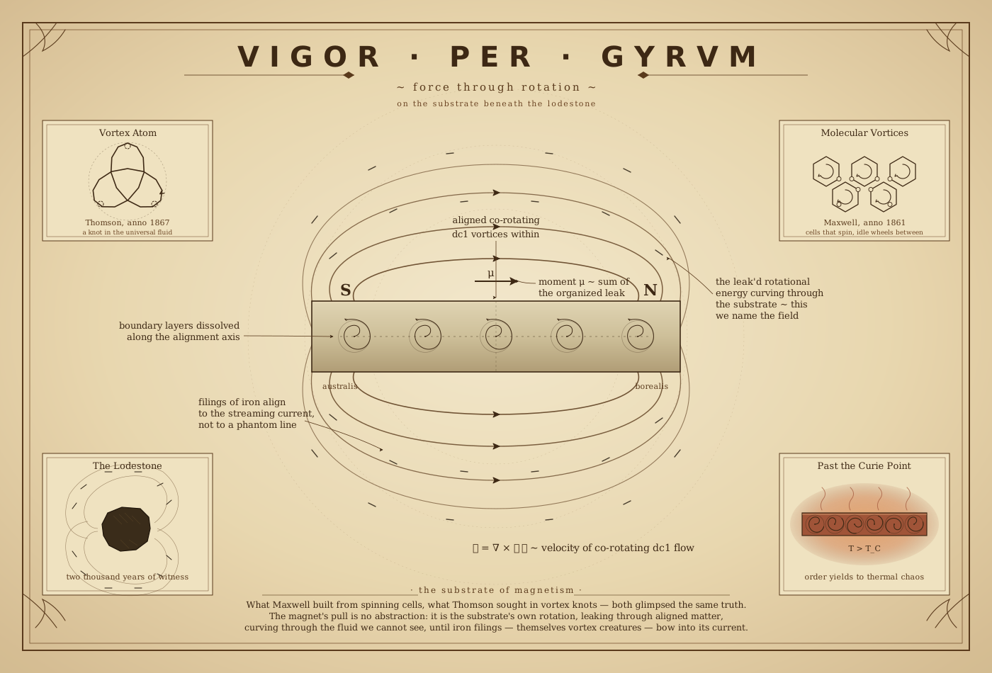
The Oldest Clue
Lodestones were the first evidence that something invisible organizes itself across macroscopic distances. A chunk of magnetite pulls iron filings into arcing patterns that extend well beyond the stone’s surface. The patterns are stable, directional, and strong enough to do mechanical work. For two thousand years, the question was: what is reaching out from inside the stone?
Thomson and Maxwell almost had it. In 1867, Thomson proposed the vortex atom — matter as stable knots of circulation in an all-pervading fluid.1 Maxwell, six years earlier, had built his entire theory of electromagnetism on a mental model of “molecular vortices” — spinning cells of fluid separated by idle wheels that transmitted angular momentum between neighbors.2 The idle wheels were his electrons. The spinning cells were his magnetic field. He derived every one of his equations from this picture, then discarded the model as scaffolding.
They were closer than anyone would be for 160 years. But they couldn’t get past two problems. First, how does the fluid sustain stable vortices without dissipating? A classical viscous fluid would spin down in microseconds. Second, if the electron is a vortex, why doesn’t it immediately collapse under its own radiation? The Larmor formula says an accelerating charge radiates — and a circulating vortex is perpetually accelerating. Thomson and Maxwell had no answer. The vortex atom programme died, and physics took the algebraic path: fields without a medium, particles without internal structure, forces without a mechanism.
What they were missing was the superfluid. A superfluid does not dissipate. Its vortices are topologically protected — quantized circulation that cannot decay continuously. And a counter-rotating boundary layer at v \approx 0.776c provides exactly the reaction force that prevents collapse: the quantum potential Q = -(\hbar^2/2m)\nabla^2\sqrt{\rho}/\sqrt{\rho} is not an abstract operator but the physical back-pressure of the counter-spinning dc1 eddies at the boundary of every orbital system. Thomson’s vortex atom works if the fluid is a superfluid. Maxwell’s molecular vortices work if the spinning cells are the dc1 condensate’s own cell vortices, organized into the self-bound lattice. The idle wheels are the counter-rotating boundary layers.
Magnetism is where this picture becomes most directly tangible. In a magnet, the substrate’s organized rotational energy does exactly what Maxwell imagined — it leaks out of aligned orbital systems and pushes or pulls on the aligned orbital systems of nearby matter. The “field lines” that iron filings trace are not abstract mathematical constructions. They are the streamlines of organized co-rotating dc1 flow, leaked through the boundary layers of trillions of aligned atomic orbital systems, curving from one pole to the other along the lowest-energy path through the substrate.
What a Magnetic Moment Is
An isolated atom has orbital systems — electrons — whose co-rotating dc1 flows carry angular momentum. Each electron’s flow has a chirality (spin direction relative to its orbital axis) and an orbital orientation. In most atoms, these orientations are distributed so that the net co-rotating flow, averaged over the atom’s boundary, is approximately zero. The atom leaks rotational energy isotropically through its boundary layers, and there is no preferred direction.
A magnetic moment appears when this cancellation is incomplete. In iron (Fe), the 3d shell holds six electrons in a configuration where four of the five 3d sub-orbitals each carry one electron with the same spin orientation (Hund’s first rule), and the fifth carries two. The net result: four unpaired spins, four units of co-rotating flow all pushing in the same direction through the atom’s boundary. The atom becomes a directed source of leaking rotational energy.
In the substrate picture, the magnetic moment \boldsymbol{\mu} is the vector sum of the organized co-rotating dc1 flow leaking through an atom’s outer boundary:
\boldsymbol{\mu} = -g_J \mu_B \mathbf{J}
where \mathbf{J} is the total angular momentum (orbital plus spin), \mu_B = e\hbar/(2m_e) is the Bohr magneton, and g_J is the Landé g-factor. The standard expression is unchanged. What changes is the physical content: \mathbf{J} is the net organized co-rotating dc1 circulation about the atom’s axis, \mu_B is the quantum of rotational energy leak per unit of boundary-layer angular momentum, and g_J encodes how efficiently the internal orbital and spin circulations couple to the external leak through the boundary geometry.
The magnetic field \mathbf{B} that surrounds a magnetic moment is the velocity field of the leaked co-rotating dc1 flow. Maxwell’s equations describe this flow exactly, because they are the equations of the substrate’s organized response — the acoustic geometry of a superfluid whose co-rotating currents have been given a preferred direction by an asymmetric source.
From Atoms to Magnets: The Exchange Interaction
A single iron atom has a magnetic moment, but a single iron atom does not make a magnet. Magnetism at the macroscopic scale requires the alignment of moments across billions of atoms. The question is: what makes neighboring atoms prefer to align their co-rotating flows in the same direction?
The standard answer is the exchange interaction — a quantum mechanical effect arising from the antisymmetry of the electronic wavefunction under particle exchange. Two electrons on neighboring iron atoms, each with unpaired 3d spins, have their energies shifted by the exchange integral J_{ex}:
\hat{H}_\text{ex} = -2J_{ex}\,\hat{\mathbf{S}}_1 \cdot \hat{\mathbf{S}}_2
When J_{ex} > 0 (ferromagnetic), parallel spins are energetically favored. When J_{ex} < 0 (antiferromagnetic), antiparallel spins are lower in energy.
The substrate picture gives this a mechanism. Two neighboring atoms in a crystal share a region of substrate between their outer boundary shells. Each atom’s co-rotating dc1 flow leaks through its boundary into this shared region. If both atoms’ flows leak with the same chirality (parallel spins), the flows in the shared region are co-rotating — they reinforce each other, and the boundary between them partially dissolves. This is the same boundary dissolution that creates conduction channels in metals (conductors). The dissolved boundary is lower in energy than two intact boundaries, because maintaining a counter-rotating boundary layer costs rotational kinetic energy.
If the two atoms’ flows leak with opposite chirality (antiparallel spins), the flows in the shared region are counter-rotating. They create an additional boundary layer — a new counter-rotating interface between the two atoms’ flows. This costs energy. The energy difference between the dissolved-boundary (parallel) configuration and the additional-boundary (antiparallel) configuration is the exchange energy J_{ex}.

Antiferromagnetic order is the magnetic face of the substrate’s own preferred pairing. The lattice locks like objects into an anti-phase relationship — the Cooper pair and the lattice’s anti-phase breath, where each vortex is shadowed by a counter-rotating partner sharing a seam. An antiferromagnet is that pairing made macroscopic and static: neighbouring moments lock counter-rotating, sharing the additional boundary the substrate elsewhere prefers to build, while a ferromagnet is the in-phase configuration that dissolves the boundary instead. The same two readings — in-phase merge versus anti-phase shared seam — that decide whether two electrons pair, two nucleons bind, or two lattice cells breathe together, decide the sign of J_{ex}.
Whether J_{ex} is positive or negative depends on the geometry. In iron, the 3d orbitals on neighboring atoms are close enough that their leaked flows overlap significantly in the shared region, and the overlap geometry favors co-rotating merging. In manganese oxide (MnO), the Mn–O–Mn superexchange pathway routes the leaked flow through the oxygen’s 2p boundary, which reverses the chirality — the flow arrives at the second Mn atom with opposite chirality, favoring antiparallel alignment. The standard Goodenough-Kanamori rules for the sign of the exchange interaction are, in substrate language, rules about whether the boundary pathway between two atoms preserves or reverses the chirality of the leaked co-rotating flow.
Anti-Phase Self-Screening
The antiferromagnetic case has a consequence that reaches past magnetism into the nature of the vacuum itself. When neighboring moments lock anti-parallel, the substrate’s leaked co-rotating flow is arranged in a checkerboard — every source shadowed by an equal, opposite source one cell away. Such an arrangement does not merely fail to reach; it actively hides itself, and the effect is quantitative.
Vokoun and colleagues measured exactly this in a benchtop system: two arrays of NdFeB cylindrical magnets on a square grid, with first-neighbor magnetization anti-parallel.3 Because neighboring dipoles cancel, the leading surviving interaction between two such arrays is not dipole–dipole but quadrupole–quadrupole, and the collective field decays correspondingly fast. Their infinite-array result gives the force as a sum over odd indices,
F \;\propto\; \sum_{i,j\,\text{odd}} \frac{J_1^2(\rho_{ij})}{\rho_{ij}^2}\,\sinh^2(\tau\rho_{ij})\,e^{-\zeta\rho_{ij}}, \qquad \rho_{ij}=\frac{\pi}{2}\sqrt{i^2+j^2},
the same J_1 Bessel structure that governs the modon’s boundary match. The lowest term sets a screening length: \rho_{11}=\pi/\sqrt2\approx2.22, so across one lattice constant (\zeta=2 in their units) the collective field falls by e^{-4.44}\approx1\%. The paper states the corollary plainly — “the increasing size of the larger set does not matter too much… a consequence of the rapid decay of the field generated by the outer regions” — the outer cells contribute almost nothing. An anti-phase array is self-screening: its leak is real, but bottled within one cell.
Contrast the aligned (parallel) array, whose sum runs over even indices and keeps the q=0 term: it reaches. In Vokoun’s numbers the anti-parallel contact force is the stronger of the two (21.3 N against 1.8 N to an infinite background), yet it is gone within a cell while the parallel field carries far. One arrangement bit — parallel or anti-phase — decides whether the same substrate leak reaches macroscopically or vanishes within a cell. A permanent magnet is the parallel choice made coherent across 10^{23} atoms; the substrate vacuum is the anti-phase choice made universal.
This is the magnetostatic face of why the vacuum is invisible. The stealth vacuum chapter shows the substrate hides because its structure factor vanishes at long wavelengths, S(\mathbf q\to0)\to0, with the surviving weight pushed up to a single ring at the cell scale q\approx2\pi/\xi. Anti-phase self-screening is that statement read in multipole language: cancelling the dipole removes the small-\mathbf q (long-range) weight and leaves the quadrupole at the cell scale — the ring. The anti-phase breath is not only why the vacuum is quiet; it is the mechanism that makes the vacuum hyperuniform — an independent route to the same S(\mathbf q\to0)\to0 that the domain-glass geometry reaches from the other side.
Vokoun’s array is the static projection — the checkerboard frozen in resin. Its dynamical counterpart is already in this chapter: the antiferromagnetic magnon (below), two sublattices precessing in anti-phase at terahertz frequencies, held by the same exchange coupling. The static checkerboard and the breathing magnon are the two halves of the substrate’s own anti-phase pair — standing, a Cooper pair; propagating, a photon — made macroscopic and measurable in an ordinary antiferromagnet.
Domains: The Substrate’s Compromise
If the exchange interaction favors parallel alignment, why isn’t every piece of iron a permanent magnet? Because full alignment over macroscopic distances costs energy in a different currency: the energy of the leaked co-rotating flow outside the material.
A fully magnetized crystal has all its atomic moments aligned. The co-rotating dc1 flow leaks through every boundary in the same direction, accumulates coherently, and produces a strong external field — a large volume of organized substrate flow curving from one pole to the other. This external flow carries energy: the magnetic field energy U = \frac{1}{2\mu_0}\int B^2\,dV, integrated over all space.
The substrate framework makes this cost vivid. The external field is not an abstraction — it is actual dc1 current circulating through the substrate outside the magnet. Maintaining this organized flow over macroscopic distances requires energy, because the flow must navigate the substrate’s own vortex lattice, curving through \xi-scale cells, maintaining coherence against the substrate’s natural tendency toward isotropy.
The compromise is domain structure. The crystal breaks into regions — domains — each internally aligned, but with different domains pointing in different directions. Within each domain, the exchange interaction keeps all moments parallel (low exchange energy). Between domains, the net leaking flows partially cancel (low external field energy). The domain walls — narrow transition regions where the moments rotate from one domain’s orientation to the next — cost exchange energy (the moments aren’t parallel across the wall) but save far more magnetostatic energy by reducing the external field.
The domain wall width \delta_w balances the two costs:
\delta_w = \pi\sqrt{\frac{A}{K_u}}
where A is the exchange stiffness (energy cost of misaligning neighboring moments, proportional to J_{ex}) and K_u is the magnetocrystalline anisotropy (energy cost of pointing away from the crystal’s preferred axis). In iron, \delta_w \approx 40 nm — about 150 atomic spacings. The moments rotate smoothly through the wall, each one slightly tilted from its neighbor, in a Bloch wall spiral.
In substrate language, the domain wall is a region where the organized co-rotating leak undergoes a smooth chirality rotation. The wall width is set by the competition between boundary dissolution energy (which penalizes any misalignment between neighbors) and the crystal’s coupling to the substrate’s sheet structure (which penalizes orientations away from the easy axis). The wall itself is a helical co-rotating flow channel — a structure that the substrate supports naturally, because helical vortex configurations are stable in superfluids (the Hasimoto soliton).
The Easy Axis: What the Lattice Can Grip
That wall formula has two constants in it, and this chapter has explained one of them.
A has a mechanism: it is the exchange stiffness, and exchange is boundary dissolution — co-rotating flows in the shared region between two atoms either merge, dissolving a boundary and releasing energy, or collide and build one. K_u got a parenthesis and was left there. But it is not a minor term, and where it comes from is not obvious. Exchange depends only on the angle between two moments, so it says nothing whatever about which direction the aligned block should point relative to the crystal. It will happily align 10^{23} atoms and leave the whole assembly free to rotate. Until something pins the alignment to the lattice, a magnet has no memory, no easy axis, no coercivity, and no use — you could wipe it with a thought.
In the substrate picture the requirement is easy to state. A moment is the net co-rotating dc1 circulation leaking through the atom’s boundary. For that circulation to know which way the lattice points, the lattice’s boundaries have to press on it — which is exactly the mechanism the iron chapter describes for crystal-field splitting: a cage of external counter-rotating surfaces pressing on a folded shell, lobes pointing at a neighbour squeezed and rising, lobes pointing between them relaxing.
So single-ion anisotropy needs two things at once. It needs a circulation with a shape — a fold, aspherical, with lobes that point somewhere in particular — and it needs a lattice pressing hard enough to feel that shape.
And those two requirements fight each other, which is the whole story.
Press hard enough and you destroy the shape. In a 3d metal the crystal field is roughly an order of magnitude stronger than the spin–orbit coupling that ties a shell’s orbital circulation to its spin. The lattice wins outright: it pins the orbital circulation, freezes it, and cancels it. This is orbital quenching, L \approx 0, and what survives is very nearly pure spin. A spin is a scalar circulation with no lobes — nothing aspherical, nothing pointing, no handle. The lattice has flattened the fold, and a flattened fold offers nothing to grip.
Now bury the shell instead. A 4f shell sits under filled 5s and 5p — the same burial the iron chapter measures as linewidth and the uranium chapter reads as chemical invisibility. The crystal field that reaches it is two to three orders of magnitude weaker than its spin–orbit coupling. The lattice loses. The shell keeps its full J, keeps a large orbital component, keeps its aspherical charge cloud, and keeps its lobes. The pressing is feeble — but it is feeble pressing on something that still has a shape, and that is worth far more than hard pressing on something flat.
The magnitudes say so, across two orders of magnitude:
| Magnetic shell | Crystal field vs spin–orbit | K_1 (J/m³) | |
|---|---|---|---|
| Fe (bcc, cubic) | 3d, exposed | field wins — quenched | \approx 4.8\times10^{4} |
| Ni (fcc, cubic) | 3d, exposed | quenched | \approx -5\times10^{3} |
| Co (hcp, uniaxial) | 3d, exposed | quenched | \approx 4.5\times10^{5} |
| Nd₂Fe₁₄B (tetragonal) | 4f on Nd, buried | spin–orbit wins — unquenched | \approx 4.9\times10^{6} |
| SmCo₅ (hexagonal) | 4f on Sm, buried | unquenched | \approx 1–2\times10^{7} |
The anisotropy is largest exactly where the crystal field is weakest, because a strong crystal field destroys the thing it would otherwise grip.
That is a sign inversion in a single parameter, and the parameter is one the framework has already been using for something else entirely. Burial is a liability for chemistry, an asset for spectroscopy, and an asset again for magnetism — one depth, three instruments, and the verdicts do not agree in sign:
| Instrument | 3d — exposed | 4f — buried |
|---|---|---|
| Chemistry | variable oxidation state, catalysis, colour: a register you can address | fourteen elements chemically indistinguishable — the section’s null result |
| Spectroscopy | bands $$2000–3000 cm⁻¹ wide, colour changes completely with host | hairlines \lesssim 10 cm⁻¹, the same colour in every host — every phosphor, every Nd laser |
| Magnetism | orbital moment quenched, anisotropy feeble | orbital moment intact, anisotropy 10–100× larger — every permanent magnet worth owning |
One qualification is owed, because burial is not the only variable and pretending otherwise would overstate the case. Lattice symmetry matters independently. Cobalt’s 3d shell is quenched exactly as iron’s is, and hcp cobalt still beats bcc iron by an order of magnitude — because a cubic crystal presses on a fold from six equivalent directions and averages most of the effect away, while a uniaxial one does not. The high-anisotropy rare-earth phases are all uniaxial by construction: Nd₂Fe₁₄B tetragonal, SmCo₅ hexagonal. So the correct statement is that anisotropy is set by burial times asymmetry of the pressing, and the rare earths win on the first term while the crystal chemistry is engineered to win on the second.
The Division of Labour in a Permanent Magnet
Burial buys anisotropy, and it charges for it in the currency this chapter opened with — because a shell the lattice cannot reach is a shell the neighbours cannot reach either.
That is the same sentence read from the exchange side. J_{ex} is boundary dissolution between the leaked flows of adjacent atoms; a 4f shell screened under 5s and 5p barely leaks at all, so rare-earth–rare-earth exchange is feeble and the Curie temperatures are hopeless. Gadolinium metal orders at 293 K — room temperature, on a good day. Dysprosium manages 88 K. A magnet made of rare earth alone would have superb anisotropy and would stop being a magnet in your hand.
So the two shells the framework has been contrasting all chapter have complementary failures, and the fix is to use both at once. This is what Sagawa’s and Croat’s groups arrived at independently in 1984, and read on the ledger it is a forced division of labour rather than an alloy that happened to work:
| Component | Shell | What it supplies | Why it cannot do the other job |
|---|---|---|---|
| 2 Nd | 4f, buried | anisotropy → the easy axis, and hence coercivity | leaks too little to carry exchange |
| 14 Fe | 3d, exposed | moment and Curie temperature | quenched — no shape for the lattice to grip |
| 1 B | — | the tetragonal structure that makes the axis uniaxial | not magnetic at all |
The buried shell says which way. The exposed shell says how much, and how hot. Neither can do the other’s job, and the reason neither can is one number — how deep the shell sits — read through the two mechanisms this chapter has now given a mechanism to. Nd₂Fe₁₄B comes out at T_C = 585 K with K_1 \approx 4.9\times10^{6} J/m³, and commercial grades reach an energy product near 400 kJ/m³ against ferrite’s \sim30 and AlNiCo’s \sim80. SmCo₅ trades product for heat — around 240 kJ/m³ but T_C = 1020 K — which is why it is what you use when the motor gets hot.
The domain-wall formula then cashes the anisotropy directly, and the number is the reason these magnets are manufactured the way they are. With K_u two orders of magnitude larger, \delta_w = \pi\sqrt{A/K_u} collapses:
\delta_w(\text{Fe}) \approx 40\ \text{nm} \qquad\longrightarrow\qquad \delta_w(\text{Nd}_2\text{Fe}_{14}\text{B}) \approx 4\ \text{nm}
A wall an order of magnitude narrower is a wall that a defect of its own size can pin, and a grain below a certain size cannot host at all. In substrate language the helical chirality rotation has been compressed into a few atomic spacings, so it can no longer glide past an imperfection without paying for it. That is coercivity, and it is why the entire industrial art of rare-earth magnets is grain size and grain-boundary chemistry — grains made small and then magnetically decoupled from one another by a non-magnetic Nd-rich phase, so that reversing one does not reverse its neighbour.
It is also why dysprosium is a geopolitical problem. Nd₂Fe₁₄B’s weakness is its middling Curie temperature, so coercivity fades as a traction motor heats up, and the standard fix is to substitute dysprosium for some of the neodymium — which, on the reading above, is simply buying more burial: Dy³⁺ carries a larger single-ion anisotropy, holds the axis harder, and holds it further up in temperature. The supply chain of the electric drivetrain runs on how deeply an f-shell sits inside an atom.
And this chapter has been quietly using the result for several sections already. Vokoun’s benchtop checkerboard — the measurement behind anti-phase self-screening — is an array of NdFeB cylinders, and it can be a benchtop experiment at all because a few millimetres of this material holds its magnetization against its neighbours’ opposing fields. The buried shell is what makes the substrate’s anti-phase argument demonstrable on a table.
None of the physics here is new and the framework computes none of it. Orbital quenching by the crystal field, unquenched 4f moments, single-ion anisotropy, the 3d–4f exchange routed through the rare earth’s 5d shell, and the design logic of Nd₂Fe₁₄B are all standard magnetism, and the quantitative apparatus — crystal-field parameters, Stevens operators, first-principles anisotropy energies — is far beyond anything this framework can produce. The numbers in the tables above are measured values, not derived ones.
What the framework contributes is that K_u and J_{ex} are the same depth parameter with opposite signs, and that this is the same parameter the iron chapter reads as spectral linewidth and the uranium chapter reads as chemical invisibility. Exchange needs a shell that leaks; anisotropy needs a shell that keeps its shape; and burial trades one for the other monotonically. Read that way, a rare-earth magnet is not a fortunate alloy but the only available resolution of a genuine conflict, and the periodic table supplies one shell of each kind in adjacent blocks. The honest discount is that lattice symmetry is a second and independent variable — hcp cobalt beats bcc iron with identical burial — so the ledger orders the magnitudes only at matched site symmetry, which is the form the prediction below takes.
Why Magnets Attract and Repel
This is where the substrate picture gives intuition that field lines alone cannot.
Bring two bar magnets together, north pole to south pole. In the standard picture: the field lines from one magnet’s north connect smoothly to the other magnet’s south, the field energy decreases, and there is an attractive force. True, but why does the connection lower the energy? What is physically happening?
In the substrate picture, each magnet’s organized co-rotating dc1 flow is leaking out through the poles and curving through the substrate back to the opposite pole. When two magnets approach north-to-south, their leaked flows are co-rotating in the gap between them. The flow from magnet A’s north pole and the flow into magnet B’s south pole are moving in the same direction through the same region of substrate. Co-rotating flows in the substrate merge — their boundary dissolves, just as it does between parallel-spin electrons on neighboring atoms. The dissolved boundary releases energy, and the system moves toward the configuration that maximizes this dissolution. The magnets pull together.
Bring the same two magnets north-to-north. Now the leaked flows in the gap are counter-rotating — both flowing outward, colliding in the shared space. Counter-rotating flows create a boundary layer. The boundary costs energy. The system pushes the magnets apart to reduce the extent of this forced counter-rotation.
Magnetic attraction and repulsion are, at bottom, the same boundary dissolution and boundary creation that drives the exchange interaction between neighboring atoms — just organized coherently over macroscopic distances. The force between two magnets is the summed co-rotating flow coupling of \sim 10^{23} aligned atomic leaks, projected through the substrate between the poles.
The force law follows from this picture. The energy of the co-rotating flow in the substrate between two magnetic dipoles \boldsymbol{\mu}_1 and \boldsymbol{\mu}_2 separated by \mathbf{r} is:
U = -\frac{\mu_0}{4\pi r^3}\left[3(\boldsymbol{\mu}_1 \cdot \hat{\mathbf{r}})(\boldsymbol{\mu}_2 \cdot \hat{\mathbf{r}}) - \boldsymbol{\mu}_1 \cdot \boldsymbol{\mu}_2\right]
This is the standard dipole-dipole interaction. The substrate adds no correction to the functional form — Maxwell’s equations are the equations of the substrate’s co-rotating flow — but it provides the physical mechanism: the 1/r^3 falloff is the decay of organized co-rotating flow in a 3D substrate, and the angular dependence encodes which configurations allow boundary dissolution (attractive) versus forced boundary creation (repulsive).
The Curie Point: Thermal Destruction of Organization
Heat a permanent magnet, and its pull weakens. At the Curie temperature T_C (770°C for iron, 358°C for nickel, 1115°C for cobalt), the magnetization drops to zero and the material becomes paramagnetic — the moments are still there, but their alignment is gone.
The substrate picture of the Curie transition is direct and intuitive. Temperature is disordered kinetic energy in the substrate — chaotic dc1 flow superimposed on the organized co-rotating and counter-rotating currents. As temperature rises, this chaotic energy does two things.
First, it disrupts the boundary layers between neighboring atoms. The exchange coupling J_{ex} depends on the boundary being well-defined enough for the co-rotating flows to either merge (ferromagnetic) or oppose (antiferromagnetic). Thermal fluctuations create turbulence at the boundary — random eddies that blur the distinction between co-rotating and counter-rotating. The effective exchange coupling weakens as J_{ex}^\text{eff}(T) = J_{ex}(1 - T/T_C)^{1/2} near the critical point.
Second, thermal energy provides each moment with random torques that compete with the exchange alignment. Each atomic orbital system is being buffeted by chaotic dc1 eddies that try to randomize its orientation. Below T_C, the exchange coupling wins: the organized co-rotating leak is strong enough to keep neighbors aligned despite the buffeting. The domain structure reorganizes in response to thermal fluctuations, but the domains persist.
At T_C, the thermal chaos matches the exchange energy: k_B T_C \sim z J_{ex}, where z is the number of magnetic nearest neighbors. The Weiss mean-field estimate gives:
T_C = \frac{2z J_{ex}}{3k_B}
Above T_C, the thermal eddies win. Each atom’s co-rotating leak points in a random direction. The organized macroscopic flow disappears. The iron filings fall away.
The substrate makes the Curie transition tangible in a way that abstract statistical mechanics does not. You are watching organized rotational energy — a coherent dc1 current leaking through trillions of aligned boundary layers — drown in thermal noise. The organization doesn’t disappear gradually; it disappears critically, because alignment is a cooperative phenomenon. Each atom’s alignment depends on its neighbors’ alignment, which depends on their neighbors’ alignment. When thermal chaos breaks enough links in this chain, the entire network collapses in a narrow temperature window. The critical exponents of the ferromagnetic transition (\beta \approx 0.326 for 3D Ising, \beta \approx 0.365 for 3D Heisenberg) encode the geometry of this cooperative collapse.
The substrate framework does not change the critical exponents — those are set by the universality class of the phase transition, which depends on the symmetry of the order parameter and the dimensionality of the system, not on the microscopic mechanism. What the framework changes is the picture: the “order parameter” (magnetization) is the net organized co-rotating substrate flow per unit volume, and the “symmetry breaking” at T_C is the spontaneous emergence of a preferred flow direction from the isotropic thermal bath.
Electromagnetic Induction: Moving Boundaries, Moving Leaks
A stationary magnet has a static pattern of co-rotating dc1 flow leaking through the substrate. Move the magnet, and you move the source of that flow. The substrate’s co-rotating current must reorganize to follow the moving source, and this reorganization propagates at c — but the pattern itself moves at whatever speed you push the magnet.
When the changing co-rotating flow pattern sweeps through a conductor, it drives current. This is Faraday’s law:
\mathcal{E} = -\frac{d\Phi_B}{dt}
The substrate picture: the moving organized flow encounters the conductor’s dissolved boundary channels (the conduction band). The time-varying co-rotating substrate flow couples to the electrons’ co-rotating channels and drives them along the channel — not because a “force” acts on them, but because the substrate’s organized flow is literally pushing through the conductor’s boundary architecture, and the electrons, being co-rotating vortex systems themselves, are carried along by the flow.
The sign of the induced current (Lenz’s law) follows from boundary dynamics. The induced current creates its own organized co-rotating leak, which opposes the change in the external flow. This is the substrate’s tendency toward equilibrium: any change in the organized co-rotating pattern is resisted by the system’s inertia. The counter-flow arises because the induced current’s own leaked flow creates a counter-rotating interaction with the changing external flow — boundary creation that opposes the change.
This is the same physics as the quantum potential Q, operating at macroscopic scale. The quantum potential is the counter-rotating boundary’s reaction to changes in the co-rotating flow. Lenz’s law is the macroscopic version: organized co-rotating flow in a conductor resists changes to external organized co-rotating flow. The substrate’s boundary dynamics unify Faraday induction and quantum back-reaction as manifestations of the same counter-rotating response.
Ferrites, Spin Waves, and Magnons
In a ferromagnet below T_C, the moments are aligned but not rigid. Small perturbations propagate as spin waves — collective oscillations where each moment precesses slightly out of alignment with its neighbors, and the precession phase advances from site to site. The quanta of these spin waves are magnons.
The substrate picture of a magnon is a ripple in the organized co-rotating leak pattern. In the ground state, all atomic co-rotating flows are aligned, and the leaked flow through the substrate is uniform and steady. A magnon is a perturbation where one atom’s co-rotating flow tilts slightly, which (through exchange coupling at the boundary) tilts its neighbor’s flow, which tilts the next, propagating through the lattice as a wave. The magnon’s dispersion relation:
\omega(\mathbf{k}) = \frac{2J_{ex} S}{\hbar}\left(z - \sum_{\boldsymbol{\delta}} e^{i\mathbf{k}\cdot\boldsymbol{\delta}}\right) + \gamma \mu_0 H
where S is the spin quantum number, \boldsymbol{\delta} are nearest-neighbor vectors, \gamma is the gyromagnetic ratio, and H is the applied field. At long wavelengths (ka \ll 1), this reduces to \omega \approx Dk^2 + \gamma\mu_0 H, a gapped quadratic dispersion.
In the substrate, the quadratic dispersion arises because the restoring force is the exchange coupling between neighboring boundary layers, and the inertia is the rotational inertia of the co-rotating dc1 flow at each site. The gap \gamma\mu_0 H is the energy cost of tilting the organized leak against the external field — the substrate’s organized co-rotating flow resists being deflected, and the resistance is proportional to the flow strength (the applied field).
Magnons interact with modons (photons). A magnon can absorb a modon whose frequency matches the spin wave’s frequency, converting organized electromagnetic substrate flow into organized magnetic substrate flow. This is ferromagnetic resonance — the basis of microwave ferrite devices. The substrate picture makes the coupling intuitive: the modon’s counter-rotating vortex dipole encounters the magnon’s tilted co-rotating flows and transfers its rotational energy into the precession. The coupling is strongest when the modon’s frequency matches the precession frequency, because that is when the modon’s oscillating field is in phase with the magnon’s oscillating leak.
An antiferromagnet carries a sharper version. Its two sublattices precess in anti-phase — one leaning as the other recovers — and the exchange coupling that ties them makes the restoring force enormous, pushing antiferromagnetic resonance up into the terahertz. This is the substrate’s own anti-phase breath made macroscopic: not two electrons in a Cooper pair or two cell vortices across a seam, but two whole sublattices of \sim10^{23} moments oscillating against each other, held by the same pairing the lattice prefers. Where the static checkerboard (anti-phase self-screening) is the frozen pattern, antiferromagnetic resonance is that pattern breathing — the closest laboratory analog to the lattice’s own hum, at a frequency scale (\simTHz) set, like the hum, by the pairing energy.
Connecting to the Bridge Equation
The magnetic properties of matter connect to the bridge equation through the mutual friction parameter \alpha_{mf}. The exchange coupling J_{ex} — the energy that aligns atomic moments — is a boundary interaction between co-rotating dc1 flows mediated by the counter-rotating boundary layer. The efficiency of this coupling is set by how strongly the counter-rotating layer transmits angular momentum between neighboring co-rotating flows, which is precisely what \alpha_{mf} quantifies.
The connection is most direct for the superexchange interaction in insulators. When two magnetic ions are separated by a non-magnetic ion (Mn–O–Mn in MnO), the exchange pathway passes through the intermediate atom’s boundary. The angular momentum transfer efficiency through this boundary is:
J_{ex}^\text{super} \propto \frac{t^2}{U} \cdot g(\alpha_{mf})
where t is the hopping integral (how strongly the co-rotating flows overlap across the intermediate boundary), U is the on-site Coulomb energy (how much it costs to add an extra co-rotating quantum to one site), and g(\alpha_{mf}) is a function of the mutual friction coupling that determines how efficiently the counter-rotating boundary mediates the transfer. In the standard Anderson superexchange theory, g is implicit in the hopping and Coulomb parameters. The substrate framework makes it explicit: the counter-rotating boundary’s dynamical response — characterized by \alpha_{mf} = \sin^2\theta_W/(1 - \sin^2\theta_W) = 0.3008 — enters every magnetic coupling through the same mechanism that enters the fine structure constant, the cell occupancy, and the S_8 suppression.
This does not mean that \alpha_{mf} alone determines J_{ex} — the geometry, orbital overlap, and Coulomb repulsion are all material-specific. But the substrate-level efficiency of angular momentum transfer through a counter-rotating boundary is universal and set by the Weinberg angle. The same coupling constant that governs how the electroweak force mixes photons and Z bosons also governs, through the substrate’s boundary dynamics, how efficiently neighboring atoms in a crystal communicate their magnetic orientations.
The Substrate View of Maxwell’s Equations
Maxwell’s equations are the substrate’s co-rotating flow equations. The correspondences are:
| Maxwell | Substrate |
|---|---|
| \mathbf{E} — electric field | Gradient of co-rotating dc1 flow pressure |
| \mathbf{B} — magnetic field | Curl of organized co-rotating dc1 flow |
| \mathbf{A} — vector potential | Co-rotating dc1 flow velocity |
| \varepsilon_0 — vacuum permittivity | Substrate’s co-rotating response compliance |
| \mu_0 — vacuum permeability | Substrate’s resistance to organized co-rotating flow curl |
| c = 1/\sqrt{\varepsilon_0\mu_0} | Quasiparticle speed \hbar/(m_1\xi) |
| Displacement current \varepsilon_0\partial\mathbf{E}/\partial t | Time-varying co-rotating pressure drives dc1 flow |
| Faraday’s law | Moving organized leak reorganizes substrate flow |
| Ampère’s law | Co-rotating current sources organized dc1 flow curl |
The identity c = 1/\sqrt{\varepsilon_0\mu_0} becomes a statement about the substrate: the speed at which electromagnetic disturbances propagate depends on how easily the substrate’s co-rotating flow responds to pressure changes (\varepsilon_0) and how much inertia the organized flow carries (\mu_0). Both are material properties of the dc1 lattice, just as the speed of sound in a crystal depends on the crystal’s compressibility and density.
The unification of electricity and magnetism — Maxwell’s great achievement — is, in the substrate framework, the recognition that \mathbf{E} and \mathbf{B} are two aspects of the same co-rotating dc1 flow: \mathbf{E} describes the flow’s pressure gradient, \mathbf{B} describes its curl. A Lorentz boost mixes the two because the boost changes which part of the substrate flow appears as pressure and which appears as curl — the same physical flow, decomposed differently by a moving observer. This is why electricity and magnetism are “the same force” — they are the same substrate current, measured in different reference frames.
Why Magnetism Feels Approachable
Magnetism is perhaps the most accessible window into the substrate framework, because the substrate’s activity is macroscopically visible. You can see iron filings trace the organized flow. You can feel the attraction and repulsion. You can heat a magnet past the Curie point and feel the force vanish as thermal chaos destroys the organization.
In gravity, the substrate’s leaking rotational energy is universal and isotropic — every mass leaks, in every direction, all the time. You cannot isolate the effect or switch it off. In quantum mechanics, the substrate’s counter-rotating boundaries operate at scales far below direct observation. In cosmology, the substrate’s dynamics unfold over billions of years and billions of light-years.
But in a bar magnet, the substrate’s organized rotational energy is concentrated, directional, and switchable. You can align the leak (magnetize), randomize it (heat past T_C), reverse it (apply an opposing field), and observe the force it produces at human scale. The iron filings are not tracing an abstract mathematical field — they are tracing the actual organized dc1 substrate current leaking out of aligned atomic orbital systems, curving through the lattice from north to south, and coupling co-rotationally to every magnetically susceptible boundary it encounters.
Maxwell built electromagnetism from this picture, then let it go. Thomson built the atom from this picture, then watched it die. The substrate framework picks up where they left off, with the two ingredients they were missing: a superfluid that doesn’t dissipate, and a counter-rotating boundary layer spinning at 0.776c that doesn’t collapse. Maxwell’s molecular vortices were not wrong. They were ahead of their time by 160 years.
Predictions
Exchange coupling and mutual friction. The substrate predicts that the ratio of exchange energies in structurally analogous ferromagnets and antiferromagnets (same crystal structure, different magnetic ions) should reflect the mutual friction coupling \alpha_{mf} through the boundary pathway geometry. Systematic measurements across isostructural series (perovskites, spinels, garnets) should reveal a universal scaling with the number of boundary-mediating hops, with \alpha_{mf} setting the per-hop efficiency.
Domain wall dynamics and substrate sheet structure. Domain wall velocities in thin-film ferromagnets should show a weak anisotropy (\sim 0.1–1\%) correlated with the film’s orientation relative to the galactic-frame substrate sheet normal, because the domain wall’s helical co-rotating flow channel couples to the substrate’s chirality-coherent 2D sheets. The effect should be distinguishable from magnetocrystalline anisotropy by its rotation with the lab’s orientation in the galactic frame.
Magnon-polariton coupling at the \xi scale. Magnon-polariton resonances in ferrite structures engineered at \sim 100\;\mum periodicity (\sim 3 THz) should show anomalously strong coupling compared to structures at other periodicities, paralleling the THz photonic crystal prediction in crystal optics. The substrate’s own lattice resonance should enhance the magnon-modon coupling at this scale.
Curie temperature and boundary relaxation. The substrate predicts that the ratio k_B T_C / J_{ex} should correlate not only with coordination number z but with the boundary relaxation rate of the magnetic ion’s outer shell — measurable through the linewidth of magnon resonances well below T_C. Faster boundary relaxation (broader magnon linewidth) should correspond to higher T_C/J_{ex} ratios, because the boundary’s ability to mediate cooperative alignment depends on how quickly it communicates angular momentum.
Aharonov-Bohm phase and organized substrate flow. The substrate framework predicts that the Aharonov-Bohm phase shift should be insensitive to the detailed geometry of the \mathbf{B} \neq 0 region (solenoid shape, field distribution) as long as the total enclosed flux is the same — because the electron responds to the total organized co-rotating dc1 flow circulation, which depends only on the enclosed flux by Stokes’ theorem. This is already confirmed experimentally but is here explained rather than postulated: the gauge invariance of the phase is the relabeling symmetry of the substrate’s flow.
Anisotropy and linewidth are one depth gauge read twice, and they must run opposite. Exchange needs a shell that leaks through its boundary; single-ion anisotropy needs a shell the lattice cannot flatten. Both are set by how deeply the magnetic shell sits, so at matched site symmetry, single-ion anisotropy per magnetic ion and the spectral linewidth of that ion’s own transitions must be anticorrelated — the ion with the sharpest, most host-independent lines contributing the most anisotropy and the least exchange, and the ion with the broadest, most host-sensitive bands the reverse. Retrodicted by the two ends: 3d ions give bands $$2000–3000 cm⁻¹ wide, quenched orbital moments and K_1 \sim 10^4–10^5 J/m³ with Curie temperatures near 10^3 K, while 4f ions give hairlines \lesssim 10 cm⁻¹, unquenched moments and K_1 \sim 10^6–10^7 J/m³ with rare-earth-only ordering temperatures of 293 K (Gd) and 88 K (Dy). The controlled version holds the host fixed and walks the lanthanide series, where burial changes while charge, row and site symmetry do not.
The natural intermediate is 5f, which the uranium chapter establishes as less completely buried than 4f — broader spectra, wider accessible chemistry — so actinide single-ion anisotropy should land between the 3d and 4f values at matched symmetry. That is a genuine forward test and nobody here has run it; the actinide magnetism literature is small and the sign is not obvious in advance, since 5f carries both a stronger crystal field and a stronger spin–orbit coupling than 4f. Falsified by a strongly anisotropic ion whose own transitions are broad and strongly host-dependent, by a hairline-emitting ion with negligible single-ion anisotropy at matched site symmetry, or by a rare-earth sublattice carrying exchange comparable to a 3d sublattice’s in the same structure.
Context
The crystal optics chapter showed the modon (photon) as a probe of a crystal’s boundary architecture — the refractive index as accumulated phase delay from modon-boundary coupling at every atomic site. This chapter shows the source side: how organized co-rotating dc1 flow leaks through aligned atomic boundaries to produce the magnetic field, how boundary dissolution and creation produce attraction and repulsion, and how thermal chaos at the Curie point destroys the organization.
Together, the two chapters paint a complete picture of electromagnetism in the substrate. The modon carries electromagnetic energy through the substrate at c; the organized co-rotating leak produces the static and quasi-static fields; and Maxwell’s equations are the fluid dynamics of both. The substrate’s boundary architecture — co-rotating flows, counter-rotating separators, exchange coupling through boundary dissolution — provides the physical mechanism behind every electromagnetic phenomenon, from the iron filings on a child’s toy magnet to the Aharonov-Bohm phase shift measured in an electron interferometer.
Footnotes
Thomson, W. (Lord Kelvin), “On Vortex Atoms,” Proc. Roy. Soc. Edinburgh 6, 94–105, 1867. The paper that launched the vortex atom programme, directly inspired by Helmholtz’s theorems on vortex motion in inviscid fluids.↩︎
Maxwell, J.C., “On Physical Lines of Force,” Philosophical Magazine 21–23, 1861–1862. Parts I–IV develop the full electromagnetic theory from a mechanical model of spinning vortex cells and idle-wheel particles.↩︎
D. Vokoun, G. Tomassetti, M. Beleggia, I. Stachiv, “Magnetic forces between arrays of cylindrical permanent magnets,” J. Magn. Magn. Mater. 323 (2011) 55–60. The measured array-to-array force agrees with the analytic expression to better than 10%.↩︎