The Proton Core
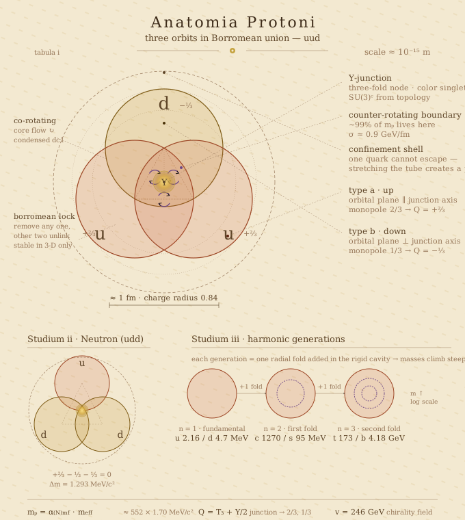
Three-Quark Orbital Topology
The previous chapter described the hydrogen atom as a six-layer flywheel and identified Layer 1 — the proton core — as a tiny region carrying 99.94% of the atom’s mass-energy. This chapter zooms in by a factor of \sim 100{,}000, from the Bohr radius (0.53 Å) down to the femtometer scale (\sim 1 fm), to examine what lives inside.
The proton’s mass budget tells the story. Two up quarks and one down quark contribute \sim 9 MeV/c^2 of bare quark mass — roughly 1% of the total. The remaining \sim 929 MeV/c^2 is what standard physics calls QCD gluon field energy. The substrate framework calls it something more intuitive: three small spinning objects confined to a tiny box, with enormously energetic counter-rotating shear layers between them. The mass is rotational energy — and the visibility-ratio picture explains where it comes from. Not from a leakier boundary: the per-boundary leak \alpha_{mf}=0.3008 is a substrate constant capped at \tfrac12, the same for the proton as for the electron. It comes from many boundaries. The nuclear number \alpha_{mf}^{(N)}\approx552 is a product N\alpha_{mf} with N\approx1836 seams, so the proton stores \sim3.12 GeV of rotational energy, shows 938 MeV of it, and keeps the other \sim2.18 GeV reactive — the same 70\% the electron hides. Why a Y-junction needs so many seams where a lone orbital needs one is § What the sheath cannot cancel.
This is the deepest inner scale of the model. The substrate has three well-separated tiers, each with its own dominant physics:
| Tier | Scale | Energy | What’s there |
|---|---|---|---|
| Outer (coherence) | \xi \approx 110\;\mum | \sim 13 meV | Soliton cell, modon/photon structure |
| Inner (electron) | r_\text{eff} \approx 150 fm | \sim 1.7 MeV | Effective quantum orbital |
| Deepest inner (nuclear) | \sim 1 fm | \sim 1 GeV | Quark orbital system complex |
The nuclear tier’s counter-rotating boundaries carry \sim 10^5 \times more energy per unit length than the electron’s, and operate in a region \sim 10^5 \times smaller. This vast scale separation is why atomic physics and nuclear physics can be treated independently — and why the proton core effectively decouples from the substrate’s outer-scale parameters.
Three quark orbital systems — two up (coral) and one down (amber) — each trace their own co-rotating flow channel in the substrate. The quarks themselves account for only about 9 MeV, roughly 1% of the proton’s total 938.3 MeV. The overwhelming majority of the mass is in those purple counter-rotating boundaries between the quark orbits.
In standard QCD, lattice calculations confirm that \sim 99\% of the proton mass comes from gluon field energy and quark kinetic energy — not from the bare quark masses. The standard explanation involves dynamical chiral symmetry breaking and the trace anomaly. In the substrate picture, it’s more intuitive: the quarks are spinning so violently in such a confined space that the counter-rotating boundary layers between them store enormous energy. That stored rotational energy is the mass.
The Universal Effective Quantum
The two-scale model revealed that the electron is built from \sim 8.3 \times 10^8 dc1 particles condensed into a single effective quantum of mass m_\text{eff} \approx 1.70 MeV/c^2, orbiting at v_\text{rot,inner}^{(e)} = 0.776c with radius r_\text{eff} \approx 150 fm. This effective quantum is not specific to the electron — it is a substrate-scale condensation unit.
The nuclear sector uses the same effective quantum, and the same per-seam leak. Both particles obey m = N\,\alpha_{mf}\,m_\text{eff} with \alpha_{mf}=0.3008 universal; the mass hierarchy is then a pure seam count, N_p/N_e = m_p/m_e \approx 1836. The proton’s three-fold junction packs \sim 1836 effective quanta into \sim 1 fm^3 — an enormous compression compared to the single effective quantum that constitutes the electron at 150 fm scale.
The figure of 552 quanta is the visible share, N\alpha_{mf} = 1836\times0.3008 = 552, which is what a scale weighs (552 \times 1.70 = 938 MeV). The stored total is the full N m_\text{eff}c^2 \approx 3.12 GeV.
This universality means the effective quantum is set by the substrate itself — by the condensation number \nu \approx 8.3 \times 10^8 and the dc1 particle mass m_1 \approx 2 meV/c^2 — not by the particle it forms. The difference between an electron and a proton is not what the building blocks are, but how many of them are organized and how tightly the counter-rotating boundaries confine them.
Why Confinement Works
The outer purple shell — the confinement boundary — is the key to why you can never isolate a single quark. In the substrate picture, this boundary is a counter-rotating layer whose energy increases as you try to stretch it. Pull two quarks apart, and the counter-rotating layer between them gets thinner and more energetic, until eventually it stores enough energy to create a new quark-antiquark pair from the substrate. You end up with two bound systems rather than a free quark.
This maps almost perfectly onto vortex reconnection in superfluid He-II, which has been studied experimentally and computationally for decades.
The three-fold Borromean topology is stable against unlinking for a deeper reason than pure geometry: it is the only three-strand configuration that is simultaneously CPT-invariant and has non-trivial color structure. Two-strand configurations (mesons) are CPT-invariant but can unlink topologically — they are metastable, not stable. Four-strand or higher configurations admit CPT-violating states that the substrate cannot sustain. Three strands, Borromean-linked, is the unique configuration where every CPT-invariant element of the braid group corresponds to a known quark assignment. Confinement is therefore not just a dynamical fact about QCD — it is a topological selection rule of the substrate, and the rule picks out exactly SU(3) as the stable three-strand interlock.
This topological argument gains independent support from the preon braid model (Mass as Rotational Energy): the three ribbon strands of the helon model map directly onto the three Y-junction branches of the vortex node, and the CPT-invariance filter on braid words reproduces the known Standard Model fermion spectrum with no spurious particles. The substrate dynamics and the braid combinatorics are describing the same topological selection.
The constant string tension
In the substrate picture, the energy per unit length of the flux tube is:
\sigma = \tfrac{1}{2}\,\rho_\text{cr}\,(\Delta v)^2 \cdot \pi\, r_\text{tube}^2
where \rho_\text{cr} is the counter-rotating layer density at the nuclear confinement scale, \Delta v is the velocity difference across the nuclear boundary, and r_\text{tube} is the tube radius. All three are set by the local substrate properties at nuclear scale, not by the tube’s length. So \sigma is constant — the tube stores exactly the same energy per femtometer whether it’s 0.5 fm or 5 fm long.
The measured value in QCD is \sigma \approx 0.18\;\text{GeV}^2 \approx 0.9\;\text{GeV/fm}. The velocity \Delta v here is the nuclear-scale orbital velocity — approaching c at these extreme energy densities, well above the electron’s inner-scale velocity of v_\text{rot,inner}^{(e)} = 0.776c and far above the outer-scale lattice velocity v_\text{rot,outer} = \omega_0\xi \approx 0.0025c.
The energy density implied by the string tension — roughly 2 GeV/fm^3 — exceeds the background substrate energy density (n_1 m_1 c^2) by sixteen orders of magnitude. This extreme compression is consistent with \sim 1836 effective quanta packed into a volume of order a few fm^3, each carrying \sim 1.70 MeV of rest energy plus comparable kinetic energy from near-luminal orbital motion.
The Y-string’s length is fixed by its energy, L_Y = E/\sigma, and this is where the count reading pays a small but real dividend. Take the stored boundary energy \approx 3.11 GeV (the 3.12 GeV total less \sim9 MeV of bare quark mass): L_Y \approx 3.11/0.9 \approx 3.46 fm, or \approx 1.15 fm per arm — comfortably larger than the flux tube’s own transverse radius of 0.38 fm ([R110]), a tube roughly three times longer than it is wide, with the quarks sitting near r_0 = 1.205 fm.
Take instead the visible energy 929 MeV, as an earlier version of this framework did: L_Y \approx 1.03 fm, or \approx 0.34 fm per arm — shorter than the tube is wide. A flux tube of radius 0.38 fm and length 0.34 fm is not a tube at all, and the quarks would sit inside the boundary meant to separate them. The geometry is incoherent, and it was a symptom of forcing stored energy to equal visible energy.
Suggestive, not decisive. Lattice’s static three-quark potential carries a large additive constant C_{3Q} that is conventionally absorbed as self-energy, so “\sigma L_\text{min} exceeds the hadron mass” is unremarkable in QCD too. The substrate’s distinctive move is to give that constant a referent — it is the reactive share, the \sim70\% that never crosses the boundary. Whether C_{3Q} extracted from lattice fits actually tracks (1-\alpha_{mf})/\alpha_{mf} times the visible energy is an unrun check, and a cheap one.
The pair creation threshold
When the tube stores enough total energy — about 2 \times 300 MeV for a light quark-antiquark pair — the substrate can reorganize. The counter-rotating boundary has enough rotational energy to spontaneously nucleate two new orbital system complexes (a quark and an antiquark) from the dc1 substrate itself. This is mass being created from pure rotational energy — E = mc^2 in its most direct form.
This is the nuclear-scale analog of the Compton oscillation that defines the electron. In the electron, energy shuttles between kinetic (contracted) and boundary (expanded) reservoirs every Compton cycle, always below the pair-creation threshold. In the stretched flux tube, the boundary energy accumulates until it crosses that threshold — the Compton-like oscillation breaks, and the energy crystallizes into new orbital system complexes.
The central junction
The most interesting feature is the region in the middle where all three orbits meet. This is a topological junction — a point where three counter-rotating boundary layers converge. It’s topologically protected, meaning you can’t smoothly deform it away. This maps onto the SU(3) color structure of QCD: the three quarks must carry three different “color charges” (red, green, blue) that sum to a color singlet. In the substrate picture, the three different orbital orientations meeting at the junction are the physical realization of that algebraic requirement — you need exactly three interlocking orbits to form a stable junction.
The figure-8 orbital topology
Each quark’s orbit traces a figure-8 path that interlocks with the other quarks’ paths. The crossing points of these figure-8 paths are where the counter-rotating boundaries are most intense and the energy density is highest — hyperbolic stagnation points where the flow field compresses and the vorticity peaks.
The neutron has the same structure but with two down quarks and one up (udd instead of uud), shifting the counter-rotating boundary energies slightly — accounting for the 1.293 MeV mass difference.
Why the nuclear boundary confines quarks
Back in the full hydrogen atom, Layer 2 (the nuclear boundary) is the outermost confinement shell — the one that faces the electron. It’s the same physics as the flux tube, but in its ground-state configuration: a closed spherical shell rather than a stretched tube. The electron never “falls into” the nucleus in a way that disrupts the quarks because Layer 2’s energy (\sim 929 MeV scale) vastly exceeds anything the electron’s 13.6 eV binding can perturb. The electron bounces off the confinement boundary like a tennis ball off a concrete wall.
This scale separation — 13.6 eV for atomic binding versus \sim 1 GeV for nuclear confinement — is why atomic physics and nuclear physics can be treated independently. In the substrate picture, they’re the same mechanism (counter-rotating boundary layers) operating at vastly different energy scales and radii. The three-tier hierarchy makes this explicit: the nuclear tier presents \sim 1836\times as many counter-rotating seams as the electron tier, each leaking the same \alpha_{mf} \approx 0.3, and each tier is effectively rigid when viewed from the tier below it.
Quark Properties in the Substrate
The table below maps each standard quark property onto its substrate framework equivalent. The confidence grades reflect the current state of the framework after integrating the visibility-ratio / braid-topology synthesis and the spin-statistics derivation.
| Property | Substrate interpretation | Status |
|---|---|---|
| Mass | Rotational KE of effective quanta at the Y-junction, leaked through counter-rotating boundaries at rate \alpha_{mf}. Bare quark mass \sim m_\text{eff}; ~99% of hadron mass is boundary energy. Quantitative: m_p = \alpha_{mf}^{(N)} \cdot m_\text{eff}, m_\text{eff} = 1.70 MeV/c^2 universal. | Strong |
| Spin | Counter-rotating boundary layer angular momentum — the half-integer winding of the boundary around the co-rotating core. The 720° return (4\pi rotation for identity) follows from the double-cover topology: SO(3) for the co-rotating flow alone, SU(2) for the co-rotating + counter-rotating system together. The 2:1 gear reduction between them is the physical content of “intrinsic angular momentum.” | Strong |
| Color charge | Topological interlocking phase at the three-fold Borromean junction. Three is the unique N giving a stable vortex junction in 3D — two can slip, four+ over-constrains. Each orbital orientation at the Y-junction is a “color”; the singlet condition (all three present) is the stability condition. Maps to SU(3) via the braid group \mathcal{B}_3. | Plausible |
| Electric charge | Solid-angle geometry of co-rotating flow at the Y-junction. Type A orientation (orbital plane contains junction axis) → monopole coupling 2/3; Type B (perpendicular) → 1/3, with sign from flow direction relative to background. Confirmed by independent ribbon-twist counting in the helon/preon model. | Strong |
| Confinement | Color flux tube = counter-rotating vortex sheet between co-rotating orbital systems. Constant string tension \sigma \approx 0.9 GeV/fm from local substrate properties. Pair creation at threshold = vortex reconnection. Maps onto experimentally verified vortex reconnection in superfluid He-II. | Strong |
| Flavor (generations) | Each generation is a radial excitation of the orbital mode at the Y-junction — the fundamental mode plus higher harmonics with additional internal counter-rotating boundary folds. Equivalently, a generation-n fermion braid threads n chirality-coherent sheets of the 3D substrate lattice, connecting to the Yukawa hierarchy via the 5D weight-lattice coordinates of the preon model. Confinement (rigid boundary) inverts the hydrogen spectrum, naturally producing steeply rising masses. The three-generation limit is the number of chirality-coherent sheets — the same calculation as the inter-sheet spacing in the bridge equation. | Plausible |
| Asymptotic freedom | At short distances (r \ll 1 fm), quarks probe the interior of each other’s co-rotating cores where the counter-rotating boundary is thinnest. The effective mutual friction coupling decreases as the boundary cross-section shrinks — quarks interact more weakly at higher energies. At large distances, the full counter-rotating vortex sheet is engaged, and the coupling grows with the sheet area until confinement takes over. | Plausible |
Mass and confinement are the two places where the substrate picture is most natural — and they’re the two aspects hardest to explain intuitively in standard QCD. Spin has been elevated from its earlier status: the double-cover derivation in Spin-Statistics and the ribbon/helon identification in Mass as Rotational Energy together give it a concrete geometric origin rather than an “intrinsic” label. Flavor, previously an open question, now has structural scaffolding from two independent directions — the radial-excitation picture at the junction and the weight-lattice / chirality-sheet picture from the braid model — though the quantitative mass ratios remain an open computation.
Color charge: a geometric answer
In QCD, the SU(3) color symmetry is imposed as an axiom — nobody explains why SU(3) rather than SU(4) or SU(2). The substrate picture offers a geometric answer: three is the minimum number of interlocking orbital systems that form a topologically stable junction in three-dimensional space. Two orbits can slip past each other. Four or more create an over-constrained junction that breaks under perturbation. Three is the sweet spot — the Borromean rings topology — and this is why baryons have exactly three quarks.
The stability analysis of N interlocking vortex tubes at a junction in 3D should show that N = 3 is the unique stable configuration. That’s a well-posed mathematical problem in vortex dynamics, connecting to Saffman’s work on vortex interactions.
Electric Charge Fractions from Junction Geometry
Why +2/3 and -1/3? In the Standard Model, these are inputs to the Gell-Mann–Nishijima formula Q = T_3 + Y/2. In the substrate framework, they emerge from the geometry of the three-fold junction.
Two distinct orbital orientations at the Y-junction
The three-fold junction has a junction axis — the line perpendicular to the plane of the Y, aligned with the proton’s spin angular momentum. Relative to this axis, there are two topologically distinct ways a quark’s orbital plane can be oriented:
Type A (the “up quark” orientation): The quark’s orbital plane contains the junction axis. Two of these can interlock at a Y-junction because they occupy two of the three branches without conflict. The co-rotating flow leaked past the quark’s counter-rotating boundary enters the junction region with a component along the junction axis — directed outward along the spin axis, the most direct path to the proton’s exterior.
Type B (the “down quark” orientation): The quark’s orbital plane is perpendicular to the junction axis, lying in the Y-plane. Its leaked co-rotating flow enters the junction region with no axial component — it flows radially in the Y-plane and must be redirected by the junction’s counter-rotating structure. This redirection is lossy: the counter-rotating boundary absorbs some of the flow, converting it to boundary energy.
The 2/3 and 1/3 ratio from solid-angle geometry
The proton’s outer confinement boundary is approximately spherical. The total co-rotating flow reaching this boundary constitutes the proton’s electric charge (+1). The fraction each quark contributes depends on its orbital orientation.
The junction flow field decomposes into spherical harmonics — the same mathematics as the hydrogen orbital angular momentum decomposition. A Type A quark’s flow pattern, projected onto spherical harmonics at the junction, has a monopole coupling of 2/3 — the orbital plane “sweeps” through 2/3 of the solid angle when it contains the axis. A Type B quark’s flow pattern has monopole coupling of 1/3 — its equatorial flow covers only 1/3 of the effective solid angle because it is confined to the equatorial plane and must redirect to reach the poles.
The sign: the Type B orientation has its orbital spin parallel to the junction axis. Its co-rotating flow opposes the background substrate flow at the equatorial boundary, creating a counter-flow. The Type B quark’s contribution to the proton’s external flow is negative — it screens rather than sources.
The charges are: Type A (up quark) Q = +2/3, Type B (down quark) Q = -1/3. Proton (uud): +2/3 + 2/3 - 1/3 = +1 ✓. Neutron (udd): +2/3 - 1/3 - 1/3 = 0 ✓.
The ledger tightens this. The solid-angle reading above (“the orbital plane sweeps 2/3 of the solid angle when it contains the axis”) is the weakest step in the derivation — it is a plausibility argument for a specific fraction, and it is what the open junction calculation is meant to confirm. The winding ledger supplies a constraint that does most of the work without it. Because charge is conserved circulation, the two orientations’ monopoles must exhaust one whole quantum between them:
|q_A| + |q_B| = 1 .
Combined with the three-fold junction’s own quantization — every arm’s share is a multiple of \tfrac13 — this forces \{|q_A|,|q_B|\} = \{\tfrac23,\tfrac13\} and admits nothing else. The mass ordering then assigns them: the heavier orientation is the one that retains more, hence escapes less, so Type B takes \tfrac13. So the fractions follow from conservation plus three-fold-ness, with the solid-angle picture demoted from load-bearing derivation to physical illustration — and the junction calculation’s job narrows correspondingly, from “produce 2/3 and 1/3” to “confirm the split is into thirds at all.”
The Gell-Mann–Nishijima connection
The formula Q = T_3 + Y/2 now has a geometric interpretation. Weak isospin T_3 maps to the quark’s orientation relative to the junction axis — Type A (orbital plane contains axis) gives T_3 = +1/2, Type B (orbital plane perpendicular) gives T_3 = -1/2. This is a binary geometric property — the orbital plane either contains the axis or it doesn’t, with continuous deformations between the two being unstable at the junction. Hypercharge Y maps to the total boundary coupling strength at the junction — Y = +1/3 for both orientations, because hypercharge measures the junction topology (three-fold → 1/3 per branch) rather than the orientation within it.
Then: Up = (+1/2) + (1/3)/2 = 2/3 ✓. Down = (-1/2) + (1/3)/2 = -1/3 ✓.
Status: This is an interpretive mapping — it assigns geometric meaning to T_3 and Y but does not yet derive the charge fractions from first principles. A rigorous derivation requires computing the monopole coefficients of the flow field at a three-fold vortex junction in 3D. If that computation gives coefficients of 2/3 and 1/3 for the two distinct orientations, the framework has a genuine prediction for fractional charge from pure geometry. The claim that fractional charge can be the winding fraction of a vortex is not itself speculative: it is measured directly in the fractional quantum Hall effect, where the Laughlin quasiparticle is a vortex in an electron condensate carrying exactly e/3 — the confined quark’s fractional charge realized, and measured, one domain over.
The mass ordering: why down is heavier than up, and by exactly how much
The Type B (down) orientation has more counter-rotating boundary surface area at the junction than Type A (up). The perpendicular orbital plane sits in the Y-plane, intersecting all three branches of the Y-junction, while the Type A orbital plane contains the axis and only intersects two branches. More boundary area → more boundary energy → more mass. That fixes the direction; the winding ledger fixes the size.
One arm, one ledger. Each arm of the junction carries one unit of circulation, and that unit has exactly two places to go. It either escapes to the confinement boundary, where its monopole is read off as the arm’s electric charge |q| — this is the preceding sections’ whole content — or it is absorbed by the arm’s counter-rotating boundary, where it becomes boundary energy, i.e. mass. Nothing else can happen to it: circulation is conserved, and the boundary is the only sink. So per arm,
\underbrace{|q|}_{\text{escapes as charge}} \;+\; \underbrace{(1-|q|)}_{\text{retained as mass}} \;=\; 1 \qquad\Longrightarrow\qquad m \;\propto\; (1-|q|),
and the mass ratio of the two orientations is fixed with nothing left over:
\frac{m_\text{down}}{m_\text{up}} \;=\; \frac{1-\tfrac13}{1-\tfrac23} \;=\; 2 .
The ledger closes across the proton’s three arms: escaped \tfrac23+\tfrac23+\tfrac13=\tfrac53, retained \tfrac13+\tfrac13+\tfrac23=\tfrac43, total 3 — three arms, three units.
Against the data. m_\text{down}/m_\text{up} = 4.70/2.16 = 2.18, and PDG’s directly-quoted ratio m_u/m_d = 0.474^{+0.056}_{-0.074} puts it in [1.89,\,2.50]. The ledger’s 2 sits comfortably inside; the naive boundary-area estimate (3 branches vs 2) gives 1.5, which is outside the interval. This is a clean comparison because quark mass ratios are renormalization-group invariant under the flavour-universal leading-order running — unlike the individual masses, there is no scheme or scale caveat to argue about. Equivalently, the statement is that |q|\,m is orientation-independent (\tfrac23\times2.16 = 1.44 MeV, \tfrac13\times4.70 = 1.57 MeV), which is the q\leftrightarrow 1-q symmetry of the ledger — and \{\tfrac23,\tfrac13\} is exactly such a pair.
The ledger also hands the junction calculation a new number to produce: the per-arm quantum M = m/(1-|q|), which comes back 6.48 MeV from the up and 7.05 MeV from the down — a 9% spread, inside the PDG errors. And it recovers the nucleon splitting, since converting a proton to a neutron re-winds one Type-A arm to Type-B: m_d - m_u = M/3 \approx 2.3 MeV, which after the Coulomb self-energy is the observed m_n - m_p = 1.293 MeV. (Numbers in scripts/nuclear_asymmetry_seam.py.)
Interactive: the arm ledger, drawn — one knot, proton or neutron, with each arm’s unit of circulation split on screen: what escapes to the shell as charge (a Type A arm’s leak exits along the junction axis; a Type B arm’s enters the equator and comes back, screening) and what the arm’s own boundary keeps as mass. The proton is a source at r_0; the neutron leaves nothing. β⁻ re-winds a Type B arm to Type A and the shed unit of counter-winding rolls off as the electron.
Note that the bare quark masses (\sim 2–5 MeV) are comparable to the effective quantum mass (m_\text{eff} \approx 1.70 MeV). This may not be coincidental — a bare quark might represent a single effective quantum (or a small number of them) whose boundary energy at the junction provides the additional mass above m_\text{eff}.
Antiquarks and mesons
An antiquark is the same orbital system with reversed chirality — the co-rotating core spins opposite to the quark. Anti-up has Type A orientation but reversed core chirality (Q = -2/3); anti-down has Type B orientation but reversed core chirality (Q = +1/3).
Mesons (quark-antiquark pairs) are two-fold junctions instead of three-fold. The orbital system and its antiparticle interlock with a single counter-rotating seam between them — topologically simpler than the baryon junction. This is why mesons are unstable: a two-fold junction in 3D can “slip” — the two orbits can unlink and separate. Baryons are stable because the three-fold Borromean topology cannot unlink without cutting.
The same fractions from ribbon twist counting
The solid-angle derivation above gives \pm 2/3 for Type A and \pm 1/3 for Type B from the junction’s monopole flow decomposition. A second, independent derivation from preon braid models arrives at the same fractions by counting ribbon twists. In the helon model, each strand of a three-ribbon braid carries an integer twist (\pm 1 or 0), and the total electric charge is one-third of the signed twist count. An up quark is \sigma_1\sigma_2^{-1}T_{12} — crossings plus two positive twists, total +2/3. A down quark is the analogous configuration with a single negative twist, total -1/3. The charge fractions are integer counts on three strands, normalized by the three-fold junction.
The two derivations are not independent computations that happen to agree. They are the same geometric fact in two languages: the solid-angle decomposition of the co-rotating flow at a three-fold junction produces the same monopole fractions that the braid combinatorics produces from three ribbons with integer twist. The substrate enforces the geometry at the fluid level; the braid math enforces it at the representation-theoretic level; both must yield \pm 2/3 and \pm 1/3 because both describe the same topological object. This is a strong internal consistency check — stronger than either derivation alone.
The Proton Charge Radius: A Second Moment of the Junction Flow
The charge fractions above are the monopole — the zeroth moment — of the co-rotating flow reaching the confinement boundary. The charge radius is the next moment of the very same field: if the boundary’s co-rotating flow sources a charge density \rho_\text{ch}(\mathbf r), then
r_p^2 \;=\; \frac{\int r^2\,\rho_\text{ch}(\mathbf r)\,\mathrm d^3 r}{\int \rho_\text{ch}(\mathbf r)\,\mathrm d^3 r},
the mean-square spread of exactly the flow whose integral gave +1. So the substrate has no separate machinery to invent here — the charge radius is the second moment of the object the previous two sections already built. That framing is what lets the framework speak to the proton radius puzzle, one of the most carefully studied discrepancies in precision physics.
The puzzle, and how it actually resolved
For a decade the proton had two charge radii that would not agree. Electronic probes — hydrogen spectroscopy and electron–proton scattering — gave r_p \approx 0.877 fm (CODATA 2014: 0.8751(61)). Muonic hydrogen, where a muon replaces the electron, gave r_p \approx 0.8409 fm ([R130] Pohl et al. 2010; [R131] Antognini et al. 2013) — about 4% smaller, a $$5σ gap that launched hundreds of papers.
The muon is the sharper ruler for a simple reason: its reduced-mass Bohr radius is $186× smaller than the electron's ($285 fm vs. 53 pm), so it spends vastly more time inside the proton, and the finite-size energy shift — scaling as m_\text{red}^3\,r_p^2 — is some \sim10^6× more sensitive to the proton’s true extent. When the electronic measurements were redone with that lesson in mind, they moved: hydrogen 2S–4P ([R132] Beyer et al. 2017, 0.8335 fm), the hydrogen Lamb shift ([R133] Bezginov et al. 2019, 0.833 fm), and the PRad electron-scattering experiment ([R134] Xiong et al. 2019, 0.831 fm) all landed near the muonic value. CODATA 2018 adopted r_p = 0.8414(19) fm. The puzzle resolved toward the smaller radius: the muon was right, and the older electronic result carried underestimated systematics.
The key experimental verdict — and the constraint any honest model must respect — is that the radius is not strongly probe-dependent. Electron and muon now agree. A framework that predicted a large intrinsic muon/electron difference would be falsified by the resolution, not vindicated by the original tension.
What the substrate contributes
The substrate does not predict a new number here; it supplies the picture the puzzle turned out to need, and it does so from structure that was already in the chapter for other reasons.
The proton is a boundary, not a point — so the muon is the honest ruler. In this framework the “charge radius” is the RMS extent of a real, diffuse counter-rotating shell (Layer 2) of finite thickness — the lattice-imaged flux tube of radius \approx 0.38 fm, junction \approx 0.47 fm ([R110]), with co-rotating flow tailing out toward the \sim 1 fm confinement boundary. A muon orbiting $$200× closer physically overlaps that shell and reads its extent directly; the electron only grazes it and infers the radius from parts-per-million spectroscopic shifts, leaving it far more exposed to systematics. The substrate therefore sides with the muonic value — which is precisely how the puzzle resolved. This is a postdiction of the resolution’s direction, read straight off “the proton is a diffuse boundary,” not a fitted number.
The number sits where the framework’s other scales say it should. 0.8414 fm falls between the flux-tube/junction core (0.38–0.47 fm) and the full nucleon size r_0 = 1.205 fm the binding-energy section already uses. The charge lives mostly in the inner Y-string network but its co-rotating flow reaches the outer boundary; the second moment of that distribution landing near 0.84 fm is what the geometry expects. A consistency check against numbers already in the paper, not a free fit.
The reframe: there is no single “proton radius”
The deeper substrate statement is structural. Because charge, mass, and spin are three distinct facets of the same boundary — co-rotating flow solid angle, counter-rotating boundary energy, and boundary circulation (the quark-property table) — the radii that probe them need not coincide, and the substrate predicts a definite ordering. The data oblige, in a way the Standard Model treats as unexplained coincidence:
| Radius (facet probed) | Measured value | Substrate facet |
|---|---|---|
| Energy / mass radius | \sim 0.4–0.5 fm (most compact) | counter-rotating boundary energy, concentrated in the Y-string core |
| Charge radius | 0.8414(19) fm | second moment of co-rotating flow at the shell |
| Magnetic radius | \sim 0.85 fm | boundary circulation (same shell) |
| Zemach radius | \sim 1.08 fm ([R131]) | charge ⊗ magnetization overlap, reaching the outer tail |
The mass is most compact (it is the dense Y-string core), charge and magnetism sit together at the shell, and the Zemach radius reaches furthest because it convolves two boundary distributions out into the tail. Four rulers, four facets of one diffuse object. Part of the historical tension came from treating “the proton radius” as a single quantity; the substrate says there are several, physically distinct, and ordered by which layer of the boundary each one weighs.
The computation this makes well-posed
This turns picture into a concrete next calculation. The charge-fraction sections propose computing the monopole of the co-rotating flow at a three-fold vortex junction to get \pm 2/3, \pm 1/3. The charge radius is the second moment of that same flow field — the same Saffman-style Y-junction calculation, carried one moment further. If it yields \sim 0.84 fm from the substrate parameters already fixed (\alpha_{mf}, the flux-tube radius, r_0), the framework has a genuine derivation rather than a postdiction. It is the same open computation as the charge fractions, and resolving one resolves both.
The substrate does not predict a probe-dependent charge radius — that would contradict the resolved data, where muon and electron now agree. What it offers is (1) a narrative postdiction of the puzzle’s resolution: the proton is a diffuse boundary, so the closer-orbiting muon is the reliable ruler and \sim 0.84 fm is the true value — the direction the field actually moved; (2) a consistency check — 0.84 fm sits between the framework’s flux-tube core (0.38 fm) and nucleon size (1.205 fm); and (3) a structural prediction — charge, magnetic, Zemach, and energy radii are distinct facets of one boundary and must be ordered (energy < charge ≈ magnetic < Zemach), which the data confirm. The genuinely predictive number — deriving 0.84 fm as the second moment of the Y-junction flow — is the same open Saffman-junction calculation flagged for the charge fractions.

The Generation Puzzle: Harmonics of the Orbital Mode
If quarks are orbital modes at a three-fold junction, then the up/down pair is the fundamental mode — the simplest standing wave pattern that satisfies the boundary conditions. The charm/strange and top/bottom pairs would be higher harmonics — more complex oscillatory patterns in the same junction topology, with more internal nodes and correspondingly higher energies.
The strange quark (Q = -1/3, like down, but m_s \approx 95 MeV) would be the first radial excitation of the Type B orientation. In the hydrogen analogy: the down quark is the n = 1 ground state of the perpendicular orbital mode, and the strange quark is n = 2 — same angular geometry but with one additional counter-rotating boundary fold inside the quark’s own orbital system. The electric charge is unchanged because charge depends on the junction orientation (Type A vs Type B), not on the internal radial structure. This is why all Type B quarks (down, strange, bottom) have Q = -1/3 and all Type A quarks (up, charm, top) have Q = +2/3 — regardless of generation.
| Generation | Type A (charge +2/3) | Type B (charge -1/3) |
|---|---|---|
| 1st | up (2.16 MeV) | down (4.7 MeV) |
| 2nd | charm (1,270 MeV) | strange (95 MeV) |
| 3rd | top (173,000 MeV) | bottom (4,180 MeV) |
The masses increase dramatically with generation because each radial excitation adds a counter-rotating boundary fold inside a confined volume. In hydrogen, the energy levels get closer together as n increases (-13.6/n^2) because the cavity is open — the outer boundary softens. In the proton’s confinement boundary, the walls are rigid — the flux tube has constant energy density. So additional internal folds are compressed, and the boundary energy per fold increases with each successive generation. This is the opposite of hydrogen, and the reason the generation masses increase so steeply rather than converging.
The same pattern should apply to leptons: the electron/muon/tau triplet may be the fundamental mode plus two harmonics of a single-fold boundary — the leptonic analog of quark generations, but without the three-fold junction that locks the charge to fractional values. In the lepton case, the single orbital system has integer charge (\pm 1) at all harmonic levels. For the charged leptons this is where the framework now gets numbers: read as the three cube-root phases of one three-fold knot, they are forced onto Koide’s Q=2/3 (a 9-ppm, zero-parameter hit) and their mass ratios — including m_\mu/m_e=206.77 — follow from a single residual phase (Three Generations from One Turning Knot).
The braid model’s independent convergence
The mass-topology synthesis provides an independent structural account of generations from the combinatorial side. The preon braid model notes that higher-generation fermions cannot fit inside \mathcal{B}_3 — they require an extended braid group with additional strands. The substrate’s interpretation is that each additional strand corresponds to penetration of an additional chirality-coherent sheet in the stacked 3D lattice. A first-generation fermion braid lives inside a single sheet (\mathcal{B}_3). A second-generation fermion braid threads two sheets (more strands, more crossings, an internal boundary fold). A third-generation braid threads three. The three-generation limit is then the statement that n = 4 sheet penetration is dynamically unstable — the same calculation as the inter-sheet spacing d in the bridge equation WIP-15. Resolving one would resolve both.
This convergence is significant: the hydrodynamic picture (radial excitations in a confined junction) and the combinatorial picture (additional braid strands from sheet penetration) arrive at the same three-generation structure from opposite starting points. They also agree on why the masses increase steeply — additional boundary folds in a rigid cavity (hydrodynamic) versus additional crossings in a higher-dimensional braid (combinatorial).
The Yukawa hierarchy as a cross-section calculation
The Standard Model parameterizes fermion masses through 13+ Yukawa coupling constants y_f, each a free parameter with m_f = y_f v/\sqrt{2} where v = 246 GeV is the Higgs VEV. The substrate framework reframes this: the Higgs VEV is the local chirality ordering of the dc1 substrate (Higgs Field), and each Yukawa coupling is the effective boundary-interface area through which the fermion’s outermost counter-rotating layer couples to that background chirality field.
The preon model’s 5D weight-lattice coordinates give each fermion’s boundary architecture an integer label — three coordinates for twist charges on the three Y-junction branches (SU(3)_c), one for net chirality along the junction axis (U(1)_{em}), one for outer-boundary handedness. Each weight-lattice point specifies a different boundary architecture, and the Yukawa coupling should be computable as a single cross-section calculation per point, using bulk substrate parameters already determined: \alpha_{mf} = 0.3008, m_\text{eff} = 1.70 MeV/c^2, r_\text{eff} = 150 fm.
This transforms the Yukawa hierarchy from a list of 13+ free parameters to a geometric calculation — one that the substrate framework has the tools to attempt, even if the computation hasn’t yet been carried out.
Status: The structural scaffolding is in place from two independent directions, and for the charged leptons the quantitative ratios are now largely in hand: the three-generations chapter reads the three families as the cube-root phases of one three-fold junction, which forces Koide’s Q=2/3 (9 ppm, no free parameter) and lands m_\mu/m_e=206.77 from a single residual phase \delta=2/9 rad. What remains is deriving that phase — and the confined-junction harmonic calculation (a Saffman-style Y-junction with Bessel matching at each arm) is exactly the computation that should produce it from first principles, and extend the clean result through the QCD-dressed quark triads.
What the Sheath Cannot Cancel: The Quadrupole Residual
The count reading leaves a question standing. If every counter-rotating boundary in the substrate leaks the same capped fraction \alpha_{mf}=0.3008, then the whole of the proton’s weight is the statement that it presents \sim1836 such boundaries where the electron presents one. That is a large number to hand-wave. This section argues that the direction of it — many rather than one — is forced by the junction’s topology, using machinery the chapter already has.
Why one boundary suffices for a lepton
The electron’s containment problem is easy, for three reasons that are the same reason:
A closed stream surface exists. A single circulation loop carrying L=\hbar is axisymmetric: core and sheath share a symmetry axis. One can therefore lay a torus around it that is everywhere tangent to the flow — a stream surface, across which the normal flux is zero identically. Containment is perfect before any dynamics is invoked, and the only thing that gets out is the transmission \alpha_{mf} across a surface that geometry already sealed.
The breath can be exactly anti-phase. The chapter on the lattice’s pairing makes the Compton oscillation lossless by an anti-phase handoff: core and sheath, two phases, exactly \pi apart. With two participants, perfect quadrature is always available.
The boundary is borrowed, not built. The electron’s sheath is the substrate’s own inter-sheet layer (Higgs Field § From Sheets to Stacking). A first-generation lepton lies inside one chirality-coherent sheet and takes its containment from the lattice for free — which is why the electron’s entire boundary budget is sub-MeV while the proton must manufacture \sim3 GeV of its own.
Why a three-fold junction has none of that
The chapter is already committed to the fact that breaks all three, and it is load-bearing elsewhere: the junction has two topologically incompatible orbital orientations. Type A planes contain the junction axis; Type B lies perpendicular to it, in the Y-plane (§ Electric Charge Fractions). That mismatch is what produces \tfrac23 and \tfrac13. Its cost is that there is no plane the object sits in — and therefore no axis for a containing surface to share.
Follow that through and each of the electron’s three advantages fails in turn:
- No invariant torus. A single ring is an integrable flow. Three mutually linked, non-coplanar vortex filaments are a three-body vortex problem — non-integrable, with chaotic advection, and the invariant tori that would serve as containment surfaces are destroyed. There exists no closed surface everywhere tangent to the junction’s flow. Nonzero normal flux is forced by topology, before transmission is even asked about. The intuitive image is right: a sheath oscillating around a knot, perpetually reshaping to catch flow lines that keep escaping where it isn’t.
- No global quadrature. The three arms sit at 2\pi/3 — the \mathbb{Z}_3 structure that Three Generations from One Turning Knot already uses. A single sheath phase cannot be anti-phase to all three arms simultaneously; at any instant it is in quadrature with one and out of it with two. The lossless two-body handoff is unavailable in principle.
- No borrowed boundary. Because Type A and Type B orientations are mutually perpendicular, the junction cannot lie within a single chirality-coherent sheet. It threads them transversally, so the lattice supplies no ready-made sheath and the object must build its own.
A containment surface that cannot be globally tangent to the flow can still be tangent locally, patch by patch. That is what a large seam count is: the number of locally-tangent patches it takes to cover a surface that admits no global tangent structure. The framework does not compute that number, and this section does not revive the phase-space-measure route that was tried and set aside in July 2026. What it does is change the kind of question the open problem asks — from “why is a coupling 500, when couplings cap at \tfrac12” (unanswerable as posed) to “how finely must a surface be subdivided before each patch is a stream surface” (a geometry question, ill-posed only in the ordinary way).
The multipole ledger: confinement is the monopole, mass is the quadrupole
There is a sharper statement available about what escapes, and it costs nothing new.
Three sources at 0, 2\pi/3, 4\pi/3 have phasors that sum to zero. So the sheath can cancel the junction’s monopole exactly. That cancellation is not a detail — it is color neutrality, the singlet condition, the reason the proton presents no strong field to the outside world. Confinement, in this language, is the statement that the \ell=0 moment of the junction is perfectly cancellable by a three-fold-symmetric sheath.
The dipole vanishes too, by the same symmetry. The first moment that cannot be cancelled is the quadrupole.
This is not a new mechanism; it is the framework’s own result read one tier down. The stealth vacuum chapter establishes that what the lattice’s anti-phase breath cannot kill is the quadrupole, bottled in the honeycomb hollow between each trio of cells, self-screening to \sim1\% within one lattice constant. The same sentence holds at the Y-junction: three-fold symmetry cancels through \ell=1 and leaves \ell=2 standing. And the multipole efficiency ladder already in the framework — leakage \propto\beta_c^{2\ell+1}, with coherent \ell=0 and \ell=1 barred by conservation and the leak skipping to \ell=2 — is the same ladder, arrived at independently for spinning nodes.
So the proton’s mass and its confinement are the two ends of one multipole ledger:
| Moment | Fate at a three-fold junction | What it is physically |
|---|---|---|
| \ell=0 monopole | cancels exactly (\mathbb{Z}_3 phasors sum to zero) | color singlet — confinement, no external strong field |
| \ell=1 dipole | cancels by the same symmetry | no strong dipole radiation |
| \ell=2 quadrupole | survives | the residual leak — the seams, hence the mass |
The consequence that reaches the binding curve
If the uncancelled residual is a quadrupole, then the seam between two nucleons is a quadrupole–quadrupole contact, and quadrupole–quadrupole coupling is orientation-dependent. The per-contact seam energy \epsilon — the framework’s one remaining nuclear debt, the absolute scale it cannot compute — is therefore not a scalar at all. It is a function \epsilon(\Omega) of the relative orientation of the two junctions’ axes.
That reframing does three things the binding-energy sections currently cannot do.
It predicts a tensor force, which the framework has otherwise been silent about. The nucleon–nucleon interaction has a large non-central tensor component; it is why the deuteron carries a 4–6\% D-state admixture and a nonzero quadrupole moment Q_d = +0.2859 fm², and why realistic NN potentials leave the deuteron unbound if the tensor coupling is switched off ([R142], [R143]). Standard nuclear physics sources it from one-pion exchange. The substrate sources it from the residual: the winding ledger’s rule “the seam binds only what it can cancel” already says the seam is a cancellation device, and the quadrupole reading says the thing left to cancel carries \ell=2 — i.e. an S–D mixing, orientation-dependent seam. The deuteron’s quadrupole moment is then the direct measurement of the junction residual, which is the most concrete observational handle this picture has.
It explains helium-4’s anomalous binding, rather than noting it. Four junctions can place their axes on a cube or tetrahedron such that all six pairwise orientations are simultaneously at the favorable angle — and that is precisely the O_h symmetry of the B=4 Skyrmion the next section already cites ([R112]). The chapter currently records the convergence between ^4He’s quantum numbers and the cubic Skyrmion as a striking agreement. The orientation reading says why: ^4He is the smallest orientation-satisfied cluster, and ^8Be is unbound (by 92 keV) because the satisfied packing does not extend.
It explains the framework’s own success pattern. A running oddity of the nuclear sections is that everything in which \epsilon cancels lands — a_S/a_V\approx1.36 from close packing, a_\text{sym}=a_V+E_F/3 from \epsilon_\text{like}=0, m_d/m_u=2 from the arm ledger — while everything requiring \epsilon itself stays open. If \epsilon = \epsilon(\Omega), that is exactly what should happen. The liquid-drop volume term uses a_V = 6\bar\epsilon with \bar\epsilon the orientation-average over \sim12 neighbours; averaging destroys the angular structure, so contact-counting ratios survive it intact while the absolute scale needs the un-averaged function nobody has written down. The debt was never a missing number. It was a missing function.
Note also that the two cancellation conditions on a seam are independent and should not be conflated. The winding condition (\epsilon_\text{like}=0: an n–p contact cancels, an n–n contact has nothing to cancel) decides which pairs bind at all. The orientation condition decides how strongly a binding pair binds. The first is the monopole ledger; the second is the quadrupole one.
The monopole-cancels / quadrupole-survives decomposition is a symmetry statement about a three-fold junction, and it is the same statement the stealth vacuum chapter makes about the lattice — so it is structurally grounded rather than newly posited. Everything downstream of it is a picture with one observational handle: if the residual is \ell=2, the NN seam must be non-central, and the deuteron’s Q_d and D-state fraction measure it. That is a genuine point of contact, and it is a place the framework could be wrong — a purely central substrate seam would be falsified by the deuteron as it stands.
What is not delivered: no computation of \epsilon(\Omega), no angular form for the seam, no derivation of the seam count N\approx1836 (the next section offers an order-of-magnitude tiling estimate, which is not the same thing), and no number for the tensor-to-central strength ratio. The concrete next calculation is the angular dependence of the interaction energy between two three-fold vortex junctions at \sim1 fm separation — the same Saffman-style junction problem already owed for the charge fractions and the charge radius, carried to a different observable. Three open problems, one calculation.
The Shape of the Knot: Three Golden Rectangles
The two pictures of the proton’s shape are the three-fold Y-string with arms at 2\pi/3, and the three-strand Borromean lock needed by the winding ledger.
To help show how the seams sit around the knot it’s worth understanding this structure.
Three rectangles, one icosahedron
Three congruent rectangles in perpendicular planes, each centered on the origin and aligned with its long axis along a different coordinate axis form a Borromean ring for any aspect ratio a/b>1. When the aspect ratio is the golden ratio, a/b=\varphi, the twelve corners are the vertices of a regular icosahedron. For the proton \varphi is important.
The corner (a,b,0) of the first rectangle has two neighbours on its own loop, at distances 2b and 2a, and its nearest corners on each of the other two loops sit at distance \sqrt{a^2+(a-b)^2+b^2}. Setting that inter-loop distance equal to the short side 2b gives a^2-ab-b^2=0, i.e. a/b=\varphi. So the golden aspect ratio is the unique shape at which the closest approach between different loops equals each loop’s own width. Every corner then has five equidistant neighbours — one on its own loop and two on each of the others — and no pair of loops is closer than the loops are to themselves.
This allows the loops to find a balance. The golden aspect ratio balances the energy across the pairs, the same geometric form of the \mathbb Z_3 symmetry the multipole ledger relies on to cancel the monopole, and it is the anti-lock ratio that refuses to let any two partners lock at the expense of the third.
One object, two axes
The Borromean rings and the Y-junction are not two models. They are one object, with a 3-fold axis that shows its color structure and a 2-fold axis that shows its charge structure.
- Down the 3-fold axis — the body diagonal (1,1,1) of the three planes — the three rectangle planes cut the viewing plane in three lines at 120^\circ. That is the Y-string: the Steiner junction with arms at 2\pi/3 that lattice QCD images ([R109], [R110]), with the junction at the icosahedron’s center. Along this axis all three loops are equivalent, the configuration the \mathbb Z_3 phasor cancellation needs.
- Down a 2-fold axis — any one of the three coordinate axes — two of the rectangle planes contain the axis and one is perpendicular to it. That is the Type A, Type A, Type B split of § Electric Charge Fractions: the uud proton, with the junction axis along the spin.
The icosahedron’s remaining axes, the 5-fold ones through the twelve corners, show that the sheath section has no borrowed boundary. Five-fold symmetry is non-crystallographic: an icosahedral cluster cannot register with any periodic lattice. This is Frank’s explanation of why icosahedral short-range order frustrates crystallization in supercooled liquids ([R201]). The substrate’s sheets are triangular arrays with three-fold and six-fold axes. A knot with five-fold axes has no orientation in which it shares a plane or an axis with the sheet lattice, so the lattice supplies no ready-made sheath. The electron, a single loop lying in one chirality-coherent sheet, borrows its containment for free; the icosahedral knot must build every seam it has. “Anti-lock” is not a metaphor here. It is the statement that the proton’s shape refuses the lattice, and the seam count is the price.
The sheath as an onion: filling the stadium
Where do \sim1836 seams sit? The radii table says the mass is most compact, at the Y-string core near 0.4–0.5 fm, while the confinement boundary reaches r_0\approx1.2 fm. Between them lies most of the proton’s volume — a marble in a stadium, if the seams were a single shell. They are not. The natural reading of the count is a layered sheath: a first triple of seams wrapping the Y-tube, each further layer folding around the flow the layer inside it could not hold, densest against the tube and thinning outward toward r_0.
Two things the ledger forces on this picture, and both matter for the wording:
- A wrap binds; it does not hide. In the visibility ledger the visible 30\% is the mass, and the 70\% is reactive and never leaves. A layer that “caught” an escaping leak and hid it would make the proton lighter. What makes the proton heavy is more stored quanta, each showing its 30\%. So a layer’s job at formation is to turn flow that would otherwise radiate away into a standing seam, and binding it is what makes it weigh. Formation catches; steady state shows.
- The layers read in parallel, not in series. If each layer filtered the layer inside it, the visible mass would fall as \alpha_{mf}^{\,N} and vanish. The mass is linear in N. So every seam’s 30\% reads through the layers outside it: a seam’s share is an inertial readout, not a flux the next layer intercepts. The onion is a geometric nesting, not a chain of filters.
With those two rules the onion pays for something the chapter has so far only tabulated. A seam density that falls with radius is a mass density that falls with radius, and the four radii are its moments: the energy radius near the tube where the layers are densest, the charge and magnetic radii at the shell where the co-rotating flow the layers bind reaches, the Zemach radius out in the thin tail. The ordering energy < charge \approx magnetic < Zemach is what a sheath that thins outward must produce. No number is claimed for the profile; the claim is that the ordering is a consequence, not a coincidence.
Interactive: the sealed core — the steady state of that onion: three golden-rectangle loops, the Y-junction where they meet, and the 1836 counter-spinning wraps nested around the quark tubes, densest at r_\text{tube} and thinning toward r_0. Seam loops draws each wrap along its own circulation; the 552 open ones (teal) leak outward and the 1284 reactive ones (purple) slosh out and back without ever leaving.
How the knot formed, and who laid the seams
The winding ledger shows the electron born with the proton as the counter-winding the substrate had to shed the instant it wound up a knot. From superfluid vortex dynamics, the event has a definite shape.
Interactive: watch the lock form — three same-chirality loops slide into overlap, blend into the three golden rectangles, and a chirped cascade of nine reconnection cusps sends Kelvin-wave crests outward; each crest folds the bath vortices it passes into counter-spinning wraps around the Y-tube, dense against the tube and thinning toward r_0, until 1836 are laid, while the whole unit of counter-winding shed at the first cusp rolls off and settles as the electron. Seam loops draws every wrap along its own circulation, the onion of nested counter-spinning lines that no single surface could replace; Two loops only is the meson, which touches, wobbles and slips apart.
Two same-chirality vortex lines pushed into overlap in the boil do not lock. They form a metastable pair, the two-fold junction for these mesons can slip apart. Three pushed into overlap can Borromean-lock, and locking three unlinked loops requires reconnections. Every reconnection launches a burst of Kelvin waves from its cusp, so the birth of a knot is a reconnection cascade with a wave train radiating outward: the same chirping undular bore the paper reads at cosmological scale, here at femtometres. That is the discharge. The whole unit of counter-winding it sheds is the electron, which settles \sim150 fm away as one loop in one sheet.
The seams are laid out in this process as close wraps at \sim1 fm and not at 150 fm, the residual the multipole ledger identified: the quadrupole flow that no three-fold sheath can cancel. At formation it is the flow the discharge keeps throwing outward. Each crest of the wave train that folds a bath vortex into a nesting eddy freezes as one more seam — the HVBK fork between aligning into a shared path and folding into a shear zone, taken the second way, over and over — until the layer is thin enough that what it still cannot hold is the quadrupole trickle the steady-state proton lives with. The sheath is the frozen wake of the discharge, and the count is how many folds it took.
§ Why a three-fold junction has none of that reframed the open problem as “how finely must the containing surface be subdivided before each patch is a stream surface.” The simplest patch hypothesis can be checked against numbers already in the chapter. Let each patch be one reduced Compton length of the total stored energy on a side, \bar\lambda_E=\hbar c/E, tiling the lateral surface of the Y-tube, whose length is fixed by the same energy, L_Y=E/\sigma, with the lattice tube radius r_\text{tube}=0.38 fm ([R110]). Because E=N\,m_\text{eff}c^2, the count closes into a fixed point with nothing free:
N=\frac{2\pi r_\text{tube}L_Y}{\bar\lambda_E^{\,2}} \quad\Longrightarrow\quad N^2=\frac{\sigma\,(\hbar c)^2}{2\pi\,r_\text{tube}\,(m_\text{eff}c^2)^3}.
| \sigma (GeV/fm) | r_\text{tube} (fm) | N | vs. 1836 |
|---|---|---|---|
| 0.90 | 0.38 | 1730 | -6\% |
| 0.94 | 0.38 | 1768 | -4\% |
| 0.98 | 0.38 | 1806 | -2\% |
| 0.94 | 0.35 | 1843 | +0.3\% |
Two readings of the same numbers. Tiling a sphere at r_0=1.205 fm instead gives N\approx4600, so the surface that gets subdivided is the tube, not the outer shell — which is what the energy radius says, and what the onion above assumes. And with m_\text{eff}=m_e/\alpha_{mf} the fixed point reads m_p/m_e\approx\sqrt{\sigma(\hbar c)^2\alpha_{mf}^3/(2\pi r_\text{tube}m_e^3)}: the mass ratio from the string tension, the tube radius, the Weinberg angle and the electron mass.
Honest sizing. This is an estimate, not a derivation, and it must not be read as reviving the set-aside route. The patch hypothesis carries all of the content; a factor of two in patch area is a factor of two in N; the end caps and the 24\%-wider junction are ignored; and \sigma and r_\text{tube} are lattice-QCD inputs rather than substrate outputs. What it shows is that the reframed geometry question, asked in its most naive form, returns the right order of magnitude with nothing tuned — and that the seams tile the Y-tube. Numbers in scripts/nuclear_seam_tiling.py.
From Nucleons to Nuclei: The Binding-Energy Curve
The preceding sections built one nucleon — three quarks at a Y-junction inside a \sim 929 MeV confinement boundary. This section assembles many nucleons into a nucleus and asks what the substrate says about the binding-energy curve: why binding energy per nucleon rises from hydrogen, peaks near iron at \sim 8.8 MeV/nucleon, and then slowly declines. The framework’s claim is that the same counter-rotating boundary physics that confines quarks also binds nucleons — one structural level up and a hundred times weaker — and that the shape of the curve is a competition between two boundary effects the framework already owns.
Two tiers of boundary: confinement versus the residual seam
The proton’s internal boundary is a flux-tube network, and lattice QCD now images its geometry directly. The static three-quark potential is well described by
V_{3Q} = -A_{3Q}\sum_{i<j}\frac{1}{r_{ij}} + \sigma_{3Q}\,L_\text{min} + C_{3Q},
where L_\text{min} is the minimal total flux-tube length connecting the three quarks through a central junction — a Y-shaped (Steiner/Fermat) tube, with the arms meeting at 2\pi/3, decisively favored over a triangle of pairwise tubes ([R109] Takahashi et al.; [R110] Bissey et al. find the Y-shape and no \Delta-shape directly in the flux distribution). This is exactly the substrate’s three-arm Y-junction. Two of its measured features matter here. First, the baryon string tension equals the mesonic one, \sigma_{3Q}\simeq\sigma_{Q\bar Q}\approx 0.89–0.98 GeV/fm ([R111] Bali) — the framework’s statement that the boundary stores a fixed energy per unit length, set by local substrate properties (§ The constant string tension), now read off the lattice. Second, the flux tube has a finite transverse size — radius \approx 0.38 fm, with the junction \approx 24\% wider ([R110]) — so the confinement boundary is a tube of counter-rotating substrate, not a mathematical line.
Binding between nucleons is a different, far weaker tier. When two nucleons approach within \sim 1 fm, their confinement boundaries — already closed, color-singlet shells — overlap only at their tails, fusing into a shared counter-rotating seam. That shared seam is the strong nuclear force (Conductors § The Strong Force as Boundary Interlocking): not a force carrier exchanged, but a structural merger of two boundary layers into one interlocking zone. The alpha-clustering literature makes the weakness precise through the Ikeda threshold rule — developed clustering requires the inter-cluster binding to be weak, because strong binding would overlap the clusters, switch on Pauli blocking, and dissolve their identity ([R115] Freer et al.). So nucleons inside a nucleus stay nearly distinct, and the hierarchy is forced: confinement \sim 929 MeV (a full Y-string) versus binding \sim 8 MeV (a residual tail overlap), the \sim 100\times suppression that QCD calls “confinement versus the residual strong force.”
Interactive: the seam — two knots on a separation slider. Their tails overlap as e^{-(d-d_0)/\lambda}; where the arm excess is opposite (p–n) the overlapping tails fuse into one counter-rotating spindle and the two shells merge — the deuteron, 2.22 MeV, about one effective quantum. n–n touches and parts with nothing to cancel; p–p is turned back at the co-rotating barrier besides.
Helium-4 as a topological unit
Two independent pictures converge on helium-4 as the fundamental building block of the curve’s light end. On the soliton side, the B=4 Skyrmion is a cubic (O_h-symmetric) topological soliton that quantizes to spin-parity 0^+ and isospin T=0 — exactly the ^4He quantum numbers — and with realistic (massive) pions the minimal-energy Skyrmions for B=8,12,16,\dots are “molecules” of B=4 cubes, reproducing the alpha-cluster ladder ^8Be=2\alpha, ^{12}C=3\alpha, ^{16}O=4\alpha ([R112] Battye–Manton–Sutcliffe). On the nuclear side, ^4He is doubly magic (Z=N=2), all spins and isospins paired into a compact 0^+ configuration — anomalously bound (28.3 MeV; 7.07 MeV/nucleon) while the next alpha-conjugate nucleus, ^8Be, is unbound ([R115], [R116]).
In the substrate these are the same statement. Baryon number in the Skyrmion picture is the topological winding of the soliton field; in the substrate it is the winding of the counter-rotating boundary — so baryon number = number of nucleons = number of closed boundaries. The alpha is the smallest boundary-minimizing closed configuration (the corrected estimate in the helium-4 fusion section), which is why it recurs as a sub-unit. The substrate’s vortex complex and the topological soliton are describing the same closed boundary from opposite ends — the same convergence the chapter already documents between the hydrodynamic and braid pictures.
The substrate semi-empirical mass formula
The empirical binding curve is captured by the semi-empirical (liquid-drop) mass formula. Mapped term by term onto boundary mechanisms, with the fitted coefficients of [R117] (Myers–Świątecki):
| Liquid-drop term | Coefficient | Substrate mechanism |
|---|---|---|
| Volume +a_V A | a_V = 15.68 MeV | saturated seam energy \times coordination number (\sim 12 neighbors, \sim 6 shared seams per interior nucleon) |
| Surface -a_S A^{2/3} | a_S = 18.56 MeV | missing seam contacts on surface nucleons (boundary deficit) |
| Coulomb -a_C \frac{Z^2}{A^{1/3}} | a_C = 0.717 MeV | same-polarity co-rotating (EM) repulsion; a_C = \tfrac35\,\alpha\hbar c/r_0 |
| Asymmetry -a_\text{sym}\frac{(N-Z)^2}{A} | a_\text{sym}\approx 28 MeV | derived: a_V + E_F/3 = 27.96 MeV — the like-nucleon seam carries no binding (winding ledger) plus exclusion |
| Pairing \pm\delta | \delta = 11/\sqrt{A} MeV | anti-phase breathing coherence (Cooper/BCS) |
Three of these are not merely relabeled — they reduce to mechanisms the framework already established, and two of the three (Coulomb and asymmetry) now come out as numbers rather than mechanisms.
Volume term = saturation = boundary locality. Why is binding extensive (proportional to A) rather than proportional to the number of nucleon pairs? Because the seam is a contact interaction whose energy is set by local substrate properties — the same locality that makes the string tension \sigma constant (§ The constant string tension). Each nucleon binds only its immediate neighbors (\sim 12 in close packing, \sim 6 shared seams), so binding per nucleon saturates at a constant no matter how large the nucleus grows. The soliton side corroborates this independently: in the BPS-Skyrme model the classical binding energy is exactly zero — energy is strictly linear in baryon number, E = E_0|B| — because the model is invariant under all volume-preserving diffeomorphisms, i.e. it is an incompressible liquid droplet ([R113] Adam et al.; the full nuclear mass formula is worked out in the soliton-side derivation below). Zero classical binding matches the \sim 0.8\% smallness of real nuclear binding, and “incompressible droplet = saturation = boundary locality” are three names for one fact.
Coulomb term from the framework’s own \alpha. The Coulomb coefficient is a_C = \tfrac35\,e^2/r_0 = \tfrac35\,\alpha\hbar c/r_0 = \tfrac35(1.44\;\text{MeV·fm})/(1.205\;\text{fm}) = 0.717 MeV — the same-polarity repulsion of co-rotating boundaries, with \alpha already derived in the substrate (Fine Structure Constant, to 1.45%) and r_0 the confinement-boundary size. So this term is a substrate quantity, not an input.
Asymmetry term as a winding balance — and the number falls out. A proton and a neutron differ by exactly the Type-A/Type-B (up/down) orientation of one junction arm, and that orientation is the arm’s net winding — the same circulation the co-rotating flow carries out as electric charge. A nucleus that is lopsided in N-Z is therefore lopsided in its internal winding tally, and it can lower its energy by re-winding arms and shedding a whole quantum of counter-winding — an electron or positron in \beta decay — until the tally rebalances. This is the winding ledger read at nuclear scale: the valley of \beta-stability is the winding tally seeking zero, and a_\text{sym} is the energy penalty for sitting off the balance point.
That mechanism turns out to be quantitative, and by the same “\epsilon cancels in the ratio” move that fixed a_S/a_V. The internucleon seam is a counter-rotating boundary: it binds by cancelling circulation across the interface. An n–p contact presents opposite Type-A/Type-B arm excess and cancels; an n–n or p–p contact presents the same winding and has nothing to cancel. So the seam energy is not one number but two, \epsilon_{np} and \epsilon_\text{like} — and the ledger says the seam binds only what it can cancel, i.e. \epsilon_\text{like}=0. Running the same close-packed contact count with two seam energies (z=12, so 6 shared seams per interior nucleon; \delta=(N-Z)/A):
B \;=\; 6A\Big[\tfrac{1-\delta^2}{2}\,\epsilon_{np} + \tfrac{1+\delta^2}{2}\,\epsilon_\text{like}\Big] \;=\; \underbrace{3A(\epsilon_{np}{+}\epsilon_\text{like})}_{a_V} \;-\; \underbrace{3(\epsilon_{np}{-}\epsilon_\text{like})}_{a_\text{sym}^\text{int}}\frac{(N-Z)^2}{A},
so a_\text{sym}^\text{int}/a_V = (\epsilon_{np}-\epsilon_\text{like})/(\epsilon_{np}+\epsilon_\text{like}) — the absolute seam scale \epsilon, the framework’s hard open piece, cancels exactly. With \epsilon_\text{like}=0 this ratio is 1: a_\text{sym}^\text{int} = a_V. The remaining half of the empirical coefficient is the exclusion cost, which is standard free-Fermi-gas physics the framework already owns through spin-statistics — expanding E/A = \tfrac35 E_F\big[(1{+}\delta)^{5/3}+(1{-}\delta)^{5/3}\big]/2 gives exactly E_F/3. Adding them:
a_\text{sym} \;=\; a_V + \frac{E_F}{3} \;=\; 15.68 + 12.28 \;=\; 27.96\ \text{MeV},
against the measured 28.06 MeV (Myers–Świątecki’s volume-symmetry coefficient, a_V\kappa with \kappa=1.79). Read backwards, the kinetic-subtracted seam ratio is \kappa_\text{int}=1.007, i.e. \epsilon_\text{like}/\epsilon_{np} = -0.003 — zero to three decimals. Zero free parameters; the only inputs are a_V, already in the table, and nuclear saturation density (scripts/nuclear_asymmetry_seam.py).
Honest sizing: the dominant uncertainty is k_F, which over its reasonable range 1.29–1.37 fm^{-1} moves the prediction across 27.2–28.7 MeV, so this is a $$2% result, not a 0.4% one. And the kinetic/interaction split is textbook nuclear physics, not framework content — what the framework contributes is why \epsilon_\text{like}=0.
The same one rule then pays for four more facts at no extra cost: the deuteron is bound while the dineutron and diproton are not; pure neutron matter is unbound (\delta\to1 sends B\to 6A\,\epsilon_\text{like}=0, which is why neutron stars are held together by gravity rather than by the strong force); the valley of \beta-stability sits at N\approx Z; and like nucleons pair, which is the pairing term below. One sentence — the seam binds only what it can cancel — and five nuclear facts follow.
One structural bonus. Because the symmetry cost rides on the same contact tally as the binding, it inherits the same surface deficit — which is precisely why Myers–Świątecki needed one \kappa multiplying both a_V and a_S, in the form E = a_V(1-\kappa I^2)A - a_S(1-\kappa I^2)A^{2/3}. It also explains the familiar convention gap: fitting a pure (N-Z)^2/A form to finite nuclei absorbs that -a_S\kappa I^2 A^{2/3} deficit, which is why the plain SEMF asymmetry coefficient is usually quoted near 23 MeV while the volume symmetry coefficient derived here is \approx28.
The soliton-side derivation: the BPS-Skyrme mass formula
This boundary-seam mass formula has a remarkably exact counterpart on the topological-soliton side, worth following because it derives the same terms analytically and reveals which one is genuinely hard. In the BPS-Skyrme model a nucleus is a soliton of baryon number B = A, and its mass is E = E_\text{sol} + E_\text{rot} + E_C + E_I ([R118] Adam, Naya, Sánchez-Guillén & Wereszczyński, 2013):
- E_\text{sol} = \tfrac{64\sqrt2\,\pi}{15}\,\mu\lambda\,B — the classical soliton mass, exactly linear in baryon number because the Bogomolny bound is saturated. This is the volume term, and it carries zero binding among the constituents — the soliton-side image of saturation, traceable to the model’s invariance under volume-preserving diffeomorphisms (an incompressible liquid). The compacton radius R_B = (2\sqrt2\,\lambda B/\mu)^{1/3} \propto B^{1/3} reproduces the nuclear-radius law.
- E_C — the electrostatic energy of the soliton’s actual charge density (topological + isospin-current), scaling as Z^2/A^{1/3}: the liquid-drop Coulomb term, derived rather than parameterized — the same co-rotating repulsion the substrate table names.
- E_\text{rot} — collective quantization of spin and isospin; the isospin piece produces a term \propto (A-2Z)^2, the asymmetry term, directly from isorotation. (The liquid-drop “asymmetry” energy is, on the soliton side, the cost of isorotating the closed configuration.)
- E_I = a_I\,i_3 — a small explicit isospin breaking for the n–p mass difference.
Three fit parameters, all natural constants of one field theory, reproduce the binding curve to excellent accuracy for heavy nuclei.
The instructive part is what the soliton model gets wrong, because it is exactly what the substrate flags as open. The minimal BPS model has no surface term: it keeps only the topological (\mathcal{L}_6) and potential (\mathcal{L}_0) terms and drops the gradient term (\mathcal{L}_2, the pion-kinetic / \sigma-model term) that would supply a -a_S A^{2/3} surface energy. As a result it overbinds light nuclei — precisely the all-surface regime where helium-4 lives — and the authors identify the missing surface energy, sourced by that dropped gradient term, as the key correction. (The asymmetry term, too, comes out with the wrong heavy-A scaling under the simplest axially symmetric soliton and is acknowledged to need better shapes.)
This is a striking convergence. Two independent frameworks — the substrate boundary-seam picture and the BPS topological soliton — arrive at the same division of labor: the volume term is clean — a saturation theorem, boundary locality on one side and the BPS bound on the other, both giving zero bulk binding — while the surface tension is the hard, not-yet-derived piece, and in both it is a gradient/boundary energy. The substrate’s seam surface tension a_S is the soliton model’s \mathcal{L}_2 contribution: the energy of the boundary where the closed configuration meets the vacuum. The two pictures agree on what is solved and on what remains.
The iron peak
The peak of B/A falls out of the competition between the surface and Coulomb terms. Writing B/A = a_V - a_S A^{-1/3} - (a_C/4)A^{2/3} - \dots (taking Z\approx A/2) and setting \mathrm{d}(B/A)/\mathrm{d}A = 0:
A_\text{peak} \approx \frac{2\,a_S}{a_C} = \frac{2(18.56)}{0.717} \approx 52,
the iron–nickel region. (The true peak, ^{62}Ni/^{56}Fe at A\approx 56–62, sits slightly higher because the valley of stability runs Z<A/2 and the asymmetry term — both dropped in this estimate — push it up.) The same ratio is, exactly, Myers–Świątecki’s fissility parameter x = a_C Z^2 A^{-1/3}/(2\,a_S A^{2/3}) = Coulomb/(2\cdotsurface) [R117]. So the peak of the binding curve (where adding nucleons stops paying) and the onset of fission (x\to 1, where Coulomb overwhelms surface tension) are the same surface-versus-Coulomb balance read at two thresholds.
The surface-to-volume ratio is fixed by close-packing geometry
The iron-peak formula needs a_S, and the absolute seam energy is the hard, still-open scale (below). But the ratio a_S/a_V asks a separate, easier question — and that ratio is what the peak actually rides on once the framework’s own a_C is in hand. Because both terms are the same per-contact seam energy \epsilon counted in two ways (interior contacts made vs. surface contacts missing), \epsilon cancels in the ratio, leaving a pure number set by the packing alone.
Counting nearest-neighbour seam contacts on a close-packed (FCC) droplet of A nucleons (scripts/nuclear_seam_geometry.py) makes this explicit. The interior coordination is 12, so each interior nucleon makes 6 shared seams and a_V = 6\epsilon — the saturation already discussed. The surface deficit, fitted as the A^{2/3} coefficient of the bond count and cross-checked by the orientation-averaged surface tension of a smooth drop, gives
\frac{a_S}{a_V} \approx 1.36 \quad\text{(smooth sphere; faceted-lattice fits } 1.37\text{–}1.6),
with zero free parameters. The empirical Myers–Świątecki value is a_S/a_V = 18.56/15.68 = 1.18. The geometric number is {\sim}15\% high, and in an informative direction: a sharp surface breaks the most possible contacts, so close-packing geometry is an upper bracket on the surface tension. The BPS-Skyrme soliton, which drops the gradient term and so carries no surface energy at all (next section), is the lower bracket at 0. The true value sits between them, fixed by the surface diffuseness — the gradient/\mathcal{L}_2 energy that softens the sharp cut — which is exactly the one piece both routes independently flag as open.
Folding the geometric ratio back into the peak (using the empirical a_V only to set the absolute scale that is still owed) sharpens, rather than loosens, the iron prediction:
A_\text{peak} = \frac{2a_S}{a_C} = \frac{2\,(1.36\times 15.68)}{0.717} \approx 59 \;\text{–}\; 63,
squarely the observed ^{56}Fe/^{62}Ni region (56–62) — and closer to it than the bare-coefficient 52, which undershoots precisely because it drops the asymmetry term. So the framework now derives not just the existence of the peak but its location from geometry, with the surface tension bracketed above (close-packing) and below (BPS) and the empirical value caught in between.
The iron peak is a substrate competition: boundary-seam surface tension (a_S — the same seam physics as the strong force) versus co-rotating electromagnetic repulsion (a_C = \tfrac35\,\alpha\hbar c/r_0, set by the framework’s derived \alpha and the nucleon size r_0). Iron sits at the bottom of the nuclear energy valley because it is the largest nucleus whose short-range surface-seam binding still outpaces accumulated long-range boundary repulsion. Of the inputs, a_C is framework-derived and the peak structure follows from it; the surface-to-volume ratio a_S/a_V\approx1.36 is now fixed by close-packing geometry (bracketing the empirical 1.18 from above, BPS-Skyrme from below), landing A_\text{peak} at 59–63. What remains only semi-quantitative is the absolute seam energy \epsilon — the per-contact scale that sets a_V and a_S individually (see Open Problems below).
Interactive: the droplet and the curve — a close-packed droplet of knots with a seam on every n–p contact and the ledger counted live: contacts made, seams missing at the surface, the co-rotating repulsion, the winding off balance, beside the liquid-drop terms and the measured binding. The chart peels the terms off the volume line, the surface deficit fading as A^{-1/3} while the repulsion grows as A^{2/3}, and the crest falls at iron. Add a neutron (no barrier), a proton or an alpha (the barrier printed, then tunnelled), or a twin nucleus — iron + iron costs 44 MeV — and watch what sticks and what parts.
The pairing term is the lattice’s breath
The pairing term \delta — the extra binding of even-even nuclei, and the magic-number bonus — is the place where the breathing-lattice insight pays off directly. Standard nuclear physics already treats nuclear pairing as a BCS phenomenon (Bohr–Mottelson–Pines): the odd-even mass staggering and the pairing gap are Cooper physics applied to nucleons. The substrate supplies the mechanism: like nucleons pair by locking their boundary breathing anti-phase, forming a shared counter-rotating seam — the very same anti-phase breathing that binds a Cooper pair (Conductors) and that builds the lattice’s counter-spinning intermediate vortex lines out of adjacent breathing sheets (Higgs Field § From Sheets to Stacking). One mechanism, three scales:
- electron Compton breath \to Cooper-pair vortex (\sim meV, \sim 100 nm)
- nucleon boundary breath \to pairing seam (\sim MeV, \sim 1 fm)
- lattice sheet breath \to intermediate vortex line (substrate scale)
Helium-4 is the doubly-magic limit of this — both of its nucleon pairs maximally anti-phase-coherent — which is why it sits a few MeV above the smooth liquid-drop value (the closed-topology bonus flagged in the fusion section). Magic numbers are boundary-shell closures: the same alternating co-/counter-rotating shell-filling that Conductors invokes for electron shells, one structural tier down.
What is a prediction, and what is interpretation
The mechanisms are strongly grounded, by three independent routes that agree: the substrate boundary-seam picture, the topological-soliton (Skyrme/BPS) picture, and the empirical liquid-drop formula all give the same structure — extensive saturating binding, a surface deficit, Coulomb erosion, and a pairing bonus. The strong force as a boundary seam is corroborated by the lattice Y-string ([R109], [R110]); saturation as incompressibility by the BPS-Skyrme bound ([R113]); pairing as anti-phase breathing by BCS nuclear pairing. The Coulomb coefficient is derived from the framework’s \alpha; the surface-to-volume ratio a_S/a_V\approx1.36 is now computed from close-packing seam geometry with no free parameters (bracketing the empirical 1.18 from above, BPS-Skyrme’s zero from below); the asymmetry coefficient is a_V + E_F/3 = 27.96 MeV against 28.06 measured, from the winding ledger’s \epsilon_\text{like}=0 plus exclusion; and the iron peak A_\text{peak}\approx 2a_S/a_C then lands at 59–63, the observed Fe/Ni region.
Of the five liquid-drop coefficients, then, two are now derived outright (a_C, a_\text{sym}), one is fixed as a ratio to the still-open scale (a_S/a_V), and the pairing term has a mechanism but not a number. Note that a_\text{sym} is derived relative to a_V — it does not need the absolute seam energy \epsilon, which is exactly why it landed while a_V itself has not.
What is not yet zero-parameter is the absolute binding scale. The volume and surface coefficients a_V,a_S separately reduce to the per-contact seam energy \epsilon (their ratio is now geometric, but \epsilon itself is not), which the framework has not yet computed from \sigma and the seam geometry. That \epsilon carries the \sim 100–300\times residual-strong-force suppression (a tiny fractional tail overlap of the confinement boundaries), the genuinely hard part. That computation — the reduction in total flux-tube length when nucleon Y-junctions merge — is the fusion-as-junction-merger open problem, and the lattice result above sharpens it into a well-posed Steiner-tree problem: the minimal connected flux-tube network spanning the 3A quarks of a cluster, versus A separate Y-strings. Tellingly, the BPS-Skyrme derivation isolates the same quantity as its one missing piece — the surface energy from the dropped gradient term — so both routes agree that the seam/surface tension is precisely what remains. Producing a_S (hence the binding scale and the exact peak) from substrate parameters is the remaining nuclear computation; the shape of the curve, and why it peaks at iron, the framework now explains.
Open Problems in Nuclear Structure
Flavor generations. The pattern of three generations with sharply increasing masses has no explanation in the standard model. Volovik’s framework suggests that multiple Fermi points in the substrate’s momentum space could give rise to multiple fermion species. The substrate picture now has structural scaffolding from two directions — radial excitations in the confined junction and chirality-sheet penetration in the braid model — but the quantitative mass ratios remain an open computation.
SU(3) \times SU(2) \times U(1) derivation. Deriving the full gauge group from substrate topology is one of the framework’s major unsolved challenges. The proton section contributes the SU(3) → three-fold junction stability argument, which is well-posed as a vortex dynamics problem. The mass-rotational-energy chapter’s identification of the “missing SU(2)_L” — not a property of the particle topology but a strain from the chirally ordered background (Higgs VEV) — narrows the remaining gap.
Charge fractions from first principles. The solid-angle argument produces the correct ratios (+2/3, -1/3) but remains an interpretive mapping until a rigorous 3D vortex junction calculation confirms the monopole coefficients. The ledger constraint |q_A|+|q_B|=1 narrows what that calculation must supply: given three-fold quantization into thirds, conservation forces \{2/3,1/3\}, so the junction solve owes only the thirds, not the specific pair. The arm ledger m\propto(1-|q|) then ties the same flow field to the quark mass ratio (m_d/m_u = 2 against a measured 2.18, PDG range [1.89, 2.50]) and hands the calculation a new target, the per-arm quantum M\approx6.8 MeV. Whether M/m_\text{eff}\approx4 is structural or coincidence is untested.
Proton charge radius from the junction flow. The charge-radius section postdicts the resolution of the proton radius puzzle (the diffuse boundary makes the closer-orbiting muon the reliable ruler, r_p \approx 0.84 fm) and predicts the ordering of the distinct facet-radii (energy < charge ≈ magnetic < Zemach). The genuinely predictive number — deriving 0.84 fm as the second moment of the co-rotating flow at the three-fold junction — is the same Saffman-style Y-junction calculation as the charge fractions, carried one moment further. Resolving one resolves both.
Universal effective quantum at nuclear scale. The algebraic identity m_\text{eff}^{(N)} = m_\text{eff}^{(e)} \approx 1.70 MeV/c^2 should be verified physically — does the dc1 condensation scale survive unmodified at nuclear energy densities, or does the extreme compression modify the condensation number \nu?
String tension from substrate parameters. Connecting \sigma \approx 0.9 GeV/fm to the substrate’s free parameters remains the key unsolved nuclear-sector problem. The dimensional estimate (\rho_\text{cr} c^2 \approx 2.3 GeV/fm^3, requiring \sim 10^{16}-fold compression of the background substrate) constrains the nuclear boundary’s local dc1 density, which could eventually link to n_1, m_1, and the nuclear \alpha_{mf}. The Boundary Energy Profile chapter frames this as the highest-leverage open piece: the string tension, the nuclear binding scale, the quark mass ratios, and the Yukawa couplings are all the same boundary energy \tfrac12\rho_\text{cr}(\Delta v)^2 A\delta with \Delta v pinned at a rim — so the single unknown function \rho_\text{cr}(\text{compression}) closes them together, and the measured \sigma is itself the zero-depth read that function must reproduce.
Yukawa coupling calculation. The weight-lattice cross-section calculation proposed above is now a concrete next step — compute the boundary-interface area for each fermion’s braid architecture projected onto the chirality field eigenmodes. Success here would collapse 13+ Standard Model free parameters to zero.
Nuclear binding scale. The substrate mass formula explains the shape of the binding-energy curve (saturation, the iron peak A_\text{peak}\approx 2a_S/a_C, the pairing bonus) and derives the Coulomb and asymmetry coefficients (a_C from \alpha; a_\text{sym}=a_V+E_F/3 from the winding ledger), but the absolute scale — the volume and surface coefficients a_V, a_S — reduces to the per-contact seam energy, not yet computed from \sigma and the merged-junction geometry. The lattice Y-string result ([R109], [R110]) sharpens this into a well-posed Steiner-tree problem (the minimal flux-tube network spanning a cluster’s 3A quarks versus A separate Y-strings); it is the same calculation as fusion-as-junction-merger.
From the Nucleus to the Lattice
The proton core completes the inward journey through the hydrogen atom’s layered architecture — from the coherence soliton at \xi \approx 110\;\mum, through the electron’s raceway at a_0, down to the three-quark junction at \sim 1 fm. The same boundary-matching mechanism operates at every scale, the same effective quantum building block appears at every tier, and the same counter-rotating boundary physics confines quarks, quantizes electrons, and structures photons.
The next chapter turns outward — to what happens when many atoms share their electrons. The boundary merger mechanism from the flywheel chapter’s exterior section (Layer 6) scales up: when exponential tails from many atoms overlap simultaneously, the result is a conductor, and when the co-rotating channels merge into a macroscopic coherent flow, the result is a superconductor.