Mass as Leaking Rotational Kinetic Energy
What Is Mass?
Mass is the most familiar number in physics and the hardest to interpret. The Standard Model’s Lagrangian has mass as a parameter you measure and plug in. General relativity has mass as the thing that sources curvature. Neither framework tells you what mass is.
The substrate framework has an answer: mass is the fraction of a vortex complex’s rotational kinetic energy that leaks through its outermost counter-rotating boundary into the surrounding substrate. It is a transmission coefficient times a stored rotational energy — a coupling efficiency, not an intrinsic quantity. Picture a flywheel spinning behind a nearly-closed shutter: the wheel holds a great deal of energy, but you feel only the sliver of wind that escapes the gap. The stored energy is far larger than the mass, and most of it is reactive — it stays bound to the particle, sloshing in and out of the region right around it instead of escaping. You cannot weigh that reactive part, but you can catch it by probing close to the particle: it deflects anything that passes near (the “scattering phase”), it bends the surrounding flow, and it fixes the precise size of the electron’s magnetic moment — the famous (g-2) anomaly. None of it ever registers on a scale, because a scale reads only what leaks out.
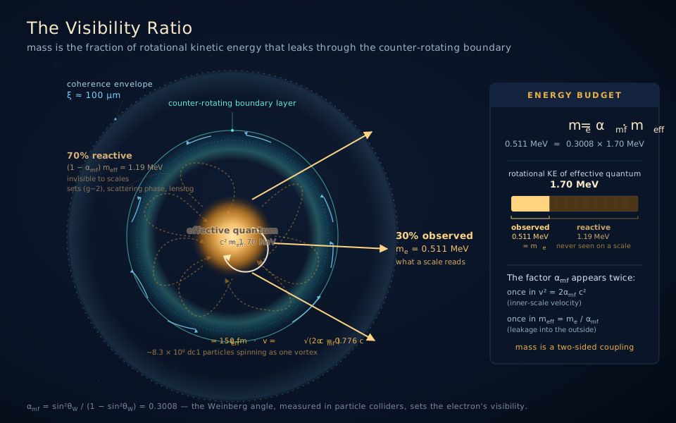
The fraction that leaks is set by a single parameter: the mutual friction coupling \alpha_{mf} = 0.3008, derived independently from the Weinberg angle (Weinberg Angle). For the electron, this identity is exact:
m_e = \alpha_{mf} \cdot m_\text{eff}, \qquad m_\text{eff} = 1.70 \text{ MeV}/c^2
The effective quantum carries 1.70 MeV of genuine rotational kinetic energy. Only 30% of it couples dissipatively to the outside substrate; the remaining 70% is reactive and invisible to mass measurements.
That 30% is not a small number by accident, and it is close to as large as it can get. The same Kopnin scattering relation that fixes it, \alpha_{mf} = \tfrac12\sin 2\delta_0, also caps it: no single counter-rotating boundary can leak more than \tfrac12, whatever its geometry. The electron’s 0.3008 already sits at 60\% of that ceiling. So the leak fraction is a substrate constant with almost no room to vary — and the way a heavy particle gets heavy cannot be by leaking harder.
It gets heavy by having more boundaries to leak through. The nuclear number that appears throughout this paper, \alpha_{mf}^{(N)}\approx552, is therefore not a coupling — it is a product, a seam count N times the same universal per-seam leak:
m \;=\; \underbrace{N}_{\text{seam count}}\cdot\underbrace{\alpha_{mf}}_{\le\,1/2,\ \text{universal}}\cdot\;m_\text{eff}, \qquad \alpha_{mf}^{(N)} \equiv N\,\alpha_{mf} .
The electron is N=1; the proton is N \approx 1836. Nucleons feel “heavy” and electrons feel “light” not because the proton hides less, but because it has vastly more aperture — while hiding the same 70\% fraction behind every one of them (Proton Core).
This chapter unpacks that picture for both particles, shows why E = mc^2 is literally the algebra of the leak, and then connects the rotational/topological view of mass to a second, independent derivation: recent combinatorial work on preon braid models that arrives at the Standard Model’s fermion spectrum from pure topology. Both descriptions converge on the same statement — particles are stable topological configurations of a rotating substrate, and their masses are the rates at which those topologies leak rotational energy to the outside world.
Electron Mass
The electron is one effective quantum — a collective vortex of \nu \approx 8.3 \times 10^8 dc1 particles — orbiting at the inner scale, dressed by a coherence region at the outer scale:
m_e \cdot c^2 = \frac{1}{2}\,m_\text{eff}\,v_\text{rot,inner}^2
where m_\text{eff} = m_e/\alpha_{mf} = 1.70 MeV/c^2 is the effective quantum mass (from C2: m_\text{eff} \cdot \alpha_{mf} = m_e) and v_\text{rot,inner} = c\sqrt{2\alpha_{mf}} = 0.776\,c (from the energy budget with N_\text{eff} = 1 and E_\text{boundary} = 0 at the contracted Compton phase).
This identity is algebraically exact: \tfrac{1}{2}(m_e/\alpha_{mf})(2\alpha_{mf}\,c^2) = m_e c^2. The electron’s rest energy equals the kinetic energy of its effective quantum at peak contraction. The factor of two in v_\text{rot,inner}^2 = 2\alpha_{mf}\,c^2 should not be read as a Lorentz factor \gamma = 2: at v = 0.776c the actual \gamma \approx 1.58, and the BEC dispersion E^2 = \mu^2 + c^2 p^2 does not map onto standard relativistic kinetic energy (the \tfrac{1}{2}mv^2 form is an energy-bookkeeping device for the quasiparticle). It is the breathing/pairing two — the radial Compton breath runs at twice the orbital frequency for an isotropic restoring dress, the temporal face of the same pairing-two that gives the lattice \xi^2 = 2\,\xi_\text{GP}^2 (The Lattice Breathes in Pairs). See Open Problems § WIP-12.
The factor \alpha_{mf} appears twice, and this is the content of the visibility-ratio thesis: once in v_\text{rot,inner}^2 = 2\alpha_{mf}\,c^2 (the orbital velocity is a fixed fraction of c set by the substrate’s coupling), and once more in m_\text{eff} = m_e/\alpha_{mf} (only \alpha_{mf} of the effective quantum’s energy reads out as mass). The squared structure of \alpha_{mf} in the observable energy balance reflects that mass is a two-sided coupling — energy must leak out of the boundary and a probe’s energy must couple in across the same boundary to register.
The orbital radius follows from one \hbar of angular momentum:
r_\text{eff} = \frac{\hbar}{m_\text{eff} \cdot v_\text{rot,inner}} = 150\;\text{fm}
| Quantity | Value | Significance |
|---|---|---|
| r_\text{eff} | 150 fm | Inner orbital scale |
| r_\text{eff} / \bar{\lambda}_C^{(e)} | \sqrt{\alpha_{mf}/2} = 0.388 | ~39% of electron reduced Compton wavelength |
| L_\text{orb} = m_\text{eff} \cdot v_\text{rot,inner} \cdot r_\text{eff} | \hbar exactly | One quantum of angular momentum |
| v_\text{rot,inner} / c | \sqrt{2\alpha_{mf}} = 0.776 | Sub-luminal, as required for BEC regime |
The Compton Oscillation: The Electron’s Heartbeat
We have been describing the electron as a whirlpool of fixed size, but that is a freeze-frame. Left to itself the vortex does something more alive: it breathes. Its energy does not sit still in one form — it sloshes back and forth between two, over and over, at a fixed rhythm. This pulse is the Compton oscillation, and it is the electron’s heartbeat.
The two forms it trades between are the two we have already met:
- Contracted phase (r_\text{eff} = 150 fm): the vortex is pulled in tight and spinning at full speed, v_\text{rot,inner} = 0.776\,c. All of the energy is in rotation.
- Expanded phase (r \sim \bar{\lambda}_C = 386 fm): the vortex has swung open, the spin has slowed, and the energy now lives in radial motion and the ripple of its boundary.
The mechanism is the oldest trick in rotational physics: a figure skater. Angular momentum is fixed — the electron carries exactly one unit, \hbar — so when the vortex pulls in it must spin faster, and when it opens out it must spin slower, just as a skater speeds up by drawing in her arms and slows by extending them. The electron does this automatically and endlessly, pumping energy from spin to boundary and back with no loss. It is a resonator, not a static ring.
The tempo is staggering. The heartbeat runs at the Compton frequency
\omega_C = \frac{m_e c^2}{\hbar} = 7.76 \times 10^{20}\;\text{rad/s} \qquad (T_C = 8.1 \times 10^{-21}\;\text{s}),
on the order of 10^{20} pulses every second. It is zitterbewegung, the “trembling motion” Schrödinger found lurking in Dirac’s equation for the free electron back in 1930. Textbook quantum mechanics treats that trembling as a mathematical curiosity — an interference between the electron’s positive- and negative-energy parts, with no physical picture attached. The substrate supplies the picture: the trembling is the vortex breathing.
How wide is the breath? Causality caps it. In one heartbeat even light travels only c\,T_C = \lambda_C = 2.43 pm, so the per-cycle breath cannot outrun the reduced Compton wavelength \bar{\lambda}_C = c/\omega_C = 386 fm. That is precisely the known amplitude of zitterbewegung — and precisely r_\text{eff}/0.388, the contracted radius scaled up by the same visibility factor that runs through this whole chapter. So the electron breathes between about 150 fm and 386 fm: a bounded pulse, not a wild swing.
This bound is worth stating carefully, because the much larger coherence envelope \xi \approx 100\;\mum is not part of this breath. That envelope is a separate, far slower structure — the static pilot-wave dress, the dc1 Compton wavelength \xi = \hbar/(m_1 c), which pulses along with the lattice at \omega_1 = m_1 c^2/\hbar, slower than the heartbeat by the mass ratio m_e/m_1 = \alpha_{mf}\nu \approx 2.5\times10^8. (An earlier reading of this framework had the electron breathing all the way out to \xi every Compton cycle, which would demand a radial speed of \sim10^8\,c; the two-mode resolution — a fast, bounded heartbeat riding inside a slow static dress — is worked out in Open Problems § WIP-12.)
The two terms in the electron’s C4 energy budget - the rotational kinetic energy and the boundary energy - are the two ends of the same pure rotation, \tfrac{1}{2}m_\text{eff}\,v_\text{rot,inner}^2, at peak contraction has become pure boundary energy, E_\text{boundary}, at peak expansion, and the two are always equal in magnitude. The trade is lossless because it is an anti-phase pair oscillation — the contracting vortex does not shed its energy into nothing; it hands it to its counter-rotating partner, the inter-sheet layer, which hands it back a quarter-cycle later (The Lattice Breathes in Pairs). What a scale reads as the electron’s mass is the RMS amplitude of this breathing mode — the time-averaged fraction of the swing’s rotational energy that leaks across the boundary each cycle.
Model the breath as a radial oscillator at fixed L=\hbar in a harmonic effective potential (V_b\propto r^2) — and the entire waveform is pinned: an ellipse of amplitude \sim\bar{\lambda}_C (the orbit turning at \omega_C/2, the breath at \omega_C), an arcsine duty cycle that leaves the electron in its expanded phase about 70\% of the time, and a time-averaged size \langle r\rangle\approx\bar{\lambda}_C. That harmonic potential is not fundamental, though — it is the effective shadow of something deeper: the Bogoliubov–de Gennes spinor’s zitterbewegung, the particle–hole (u/v) interference across a gap of m_ec^2, which is the anti-phase Cooper pairing itself (The Lattice Breathes in Pairs). Full derivation in Open Problems § WIP-12.
At the hydrogen ground state (v = c/137): the de Broglie wavelength is \lambda_B = 137\,\lambda_C = 332 pm, and 2\pi a_0 = \lambda_B exactly — Bohr quantization from a standing pilot wave.
Proton Mass
m_p \cdot c^2 = 938.3\;\text{MeV} = \underbrace{\sum m_q c^2}_{{\sim}\,9\,\text{MeV}\;(1\%)} + \underbrace{E_\text{counter-rotating boundaries}}_{{\sim}\,929\,\text{MeV}\;(99\%)}
This mirrors the standard picture where ~99% of proton mass is gluon field energy. In the substrate framework, “gluon field energy” becomes the kinetic energy of interlocking vortices — three quarks at a Y-junction, each carrying fractional charge determined by the solid-angle geometry, bound by vortex sheets with constant string tension \sigma \approx 0.9 GeV/fm. See Proton Core for the full treatment.
The visibility-ratio picture makes the \sim 99\% number intuitive rather than mysterious — but only once the nuclear number is read as a count, not a coupling. Both particles leak the same universal fraction \alpha_{mf}=0.3008 through each boundary they present, because that fraction is capped at \tfrac12 by the Kopnin relation and cannot be dialed up. What differs is N:
| Electron | Proton | |
|---|---|---|
| Seam count N | 1 | \approx 1836 |
| Per-seam leak \alpha_{mf} | 0.3008 | 0.3008 (same) |
| Stored rotational energy N m_\text{eff}c^2 | 1.70 MeV | \approx 3.12 GeV |
| Leaked (what a scale reads) | 0.511 MeV | 938.3 MeV |
| Reactive (hidden) | 1.19 MeV (70%) | \approx 2.18 GeV (70%) |
So the proton is not “mostly visible mass.” It hides 2.18 GeV — more than twice what it shows — in exactly the same proportion the electron does. What makes it heavy is that a three-fold Borromean junction cannot be contained by one boundary the way a single planar orbital can, so its containment proliferates into \sim 1836 seams; the reason it must is worked out in Proton Core § What the sheath cannot cancel.
This matters downstream. The mass-defect section predicts that binding reshapes the nucleon’s reactive ledger, observable as the EMC effect and moment quenching. That prediction requires a large reactive ledger to reshape.
The Proton–Electron Mass Ratio
The proton is about 1836 times heavier than the electron. In the Standard Model this number is brute fact: two masses are measured, and their ratio is whatever it is. The substrate framework recasts it as something more legible. Both particles are built from the same universal effective quantum, m_\text{eff} \approx 1.70 MeV/c^2 — one quantum of dc1 circulation, a property of the medium, not of either particle (Proton Core). What differs is only how many counter-rotating boundaries each particle has to present in order to contain itself. Writing the leak relation in each sector, with N the seam count and the per-seam leak \alpha_{mf}=0.3008 shared,
m_e = N_e\,\alpha_{mf}\,m_\text{eff}, \qquad m_p = N_p\,\alpha_{mf}\,m_\text{eff},
and dividing cancels both the shared quantum and the shared per-seam leak, leaving the ratio as a pure ratio of seam counts:
\frac{m_p}{m_e} = \frac{N_p}{N_e} = \frac{\alpha_{mf}^{(N)}}{\alpha_{mf}^{(e)}} \approx 1836 .
This is the same algebra as before but a different physical statement, and the difference matters. Read as a ratio of couplings it says the proton’s boundary is a thousand times leakier — which the Kopnin ceiling \alpha_{mf}\le\tfrac12 forbids outright, since the electron’s 0.3008 is already 60% of the maximum any single boundary can reach. Read as a ratio of counts it says something the framework can actually sustain: both objects leak the same 30\% per boundary, and the proton simply presents \sim1836 boundaries where the electron presents one.
The factor of 1836 is therefore not the span between an object that hides itself and one that doesn’t — both hide 70\%. It is the span between a topology that can be sealed by a single surface and one that cannot be sealed by any.
Charge is what escapes; mass is what is kept. The same 1836 sharpens a distinction that is easy to blur. The proton and electron carry exactly equal and opposite charge despite the mass gap, so charge cannot be counting seams. It counts something else: the net winding that gets out to the outside world, where a passing charge reads it through \mathbf{A} (Aharonov-Bohm § Mead’s Route). Winding is topological, so it comes in whole units, and that is charge quantization. Mass is the energy the seams keep and leak. Proton Core’s arm ledger is this split at the level of a single junction arm: each unit of circulation either escapes as charge |q| or is retained as mass 1-|q|. The neutron is the test case. Its arms escape +\tfrac23-\tfrac13-\tfrac13 = 0 net, so it presents no winding outside and carries no charge. Yet it retains more than the proton, \tfrac13+\tfrac23+\tfrac23 = \tfrac53 against \tfrac43, which is why it is the heavier of the two. Being balanced to the outside is a statement about winding. It does not mean leaking less.
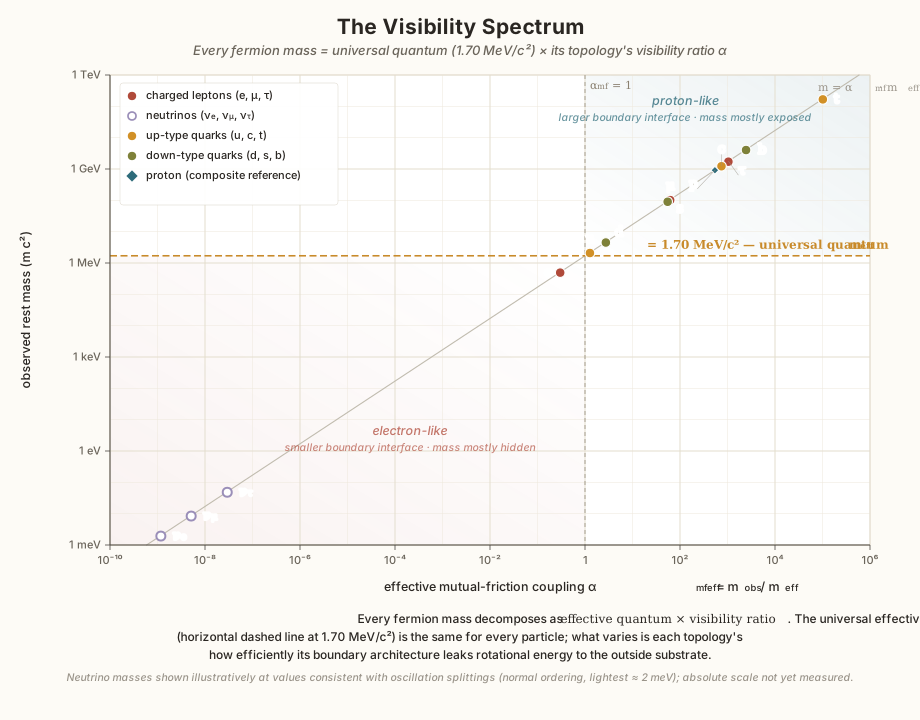
This is a reinterpretation of the number 1836. The shared quantum m_\text{eff} is itself fixed from the electron (m_\text{eff} = m_e/\alpha_{mf}, with \alpha_{mf} = \tan^2\theta_W from the Weinberg angle), so the proton’s seam count N_p = m_p/(\alpha_{mf} m_\text{eff}) = m_p/m_e is read back from the measured proton mass — the same is true for every other fermion, each of which lands on the diagonal m = \alpha_{mf}^\text{eff}\,m_\text{eff} shown in the visibility spectrum below. That single line is a unifying picture of the whole spectrum, not a table of predictions: each particle’s position encodes its mass rather than forecasting it. The genuine predictive content — computing the seam count for each sector from the topology of its vortex junction, and so deriving the mass ratios from first principles — is the open Yukawa-hierarchy and three-generation computation flagged in Proton Core and Open Problems. What the framework supplies now is the structural claim that all these ratios are one universal leak counted over different numbers of seams, and a concrete object to compute next.
Read the visibility spectrum below with that in mind: its horizontal axis is the product \alpha_{mf}^\text{eff} = N\alpha_{mf}, not a coupling. Every point above \alpha_{mf}^\text{eff}=\tfrac12 — everything from the up quark (\alpha_{mf}^\text{eff}\approx1.3) upward, which is most of the chart — is a multi-seam object, and its horizontal position is counting seams, not measuring leakiness. Only the neutrinos and the electron fall below the Kopnin ceiling, so the electron is the heaviest fermion a single counter-rotating boundary can contain. That the ceiling lands precisely in the gap between the electron and the lightest quark, rather than cutting through the middle of a family, is a structural check the diagonal picture passes rather than a fact it was fitted to. The diagonal also closes at its far end: below the neutrinos, the vacuum lattice itself occupies the N=0 row — every seam a cell owns is paired, internal, and absent from the mass ledger, which is why dark matter weighs exactly its rest-mass census, \rho_\text{DM}=n_1m_1, with no boundary surcharge (The Quiet Majority § The zero-seam row).
Why E = mc^2
Einstein’s equation is the most famous in physics, and also one of the strangest once you stop to look at it. It says that an object sitting perfectly still — a rock, an electron, anything with mass — holds an enormous reservoir of energy, and that the size of that reservoir is set by c, the speed of light. But why should the speed of light have anything to do with the energy of a stationary lump of matter? The rock isn’t going anywhere. No light is involved. Standard physics offers no answer: c is simply taken as a fundamental constant of nature, and c^2 is the fixed exchange rate between the units we call “mass” and the units we call “energy.” The equation is exact and endlessly confirmed — but it is a postulate. It tells you mass and energy are the same currency without telling you why the exchange rate should be the square of a light speed.
The substrate framework turns that postulate into a mechanism, and the mechanism is almost embarrassingly simple: nothing is ever truly at rest. What looks like a stationary electron is, close up, a whirlpool — a parcel of substrate spinning in place. A particle “at rest” is at rest only in the sense that a spinning top standing on a table is at rest: it isn’t traveling anywhere, but on the inside it is going around very fast. Its rest energy is not some abstract quantity sealed inside matter; it is ordinary rotational kinetic energy — the same energy a flywheel stores when you spin it up.
And rotational kinetic energy has a formula every physics student knows: \tfrac{1}{2}\,m\,v^2. Apply it to the electron’s internal whirlpool — a mass m_\text{eff} of spinning substrate turning at rim speed v_\text{rot,inner} — and it lands exactly on the rest energy:
\underbrace{\tfrac{1}{2}\,m_\text{eff}\,v_\text{rot,inner}^2}_{\text{flywheel energy of the spin}} \;=\; \underbrace{m_e\,c^2}_{\text{Einstein's rest energy}}
By itself that only relabels rest energy as spin energy. The reveal — the reason c^2 appears at all — is hiding in the rim speed. The inner circulation is not free to be any speed it likes. The medium has a single ceiling velocity, c, and the vortex’s rim is locked to a fixed fraction of it:
v_\text{rot,inner}^2 = 2\alpha_{mf}\,c^2, \qquad v_\text{rot,inner} = 0.776\,c .
That is where the square of the light speed enters. Substitute it into the flywheel formula and watch the pieces fall away:
\tfrac{1}{2}\,m_\text{eff}\,\big(2\alpha_{mf}\,c^2\big) \;=\; \big(\alpha_{mf}\,m_\text{eff}\big)\,c^2 \;=\; m_e\,c^2 .
The \tfrac{1}{2} and the 2 cancel; the coupling \alpha_{mf} converts the effective quantum’s mass m_\text{eff} into the observed electron mass m_e (the visibility ratio from the start of this chapter — only \alpha_{mf} of the spin energy leaks out where a scale can read it); and what remains standing is m_e c^2, letter for letter.
So E = mc^2 reads, in this framework, as a sentence about a spinning fluid rather than an axiom about matter. The c^2 is not a mysterious exchange rate handed down from the postulates of relativity — it is the flywheel’s rim speed, pinned to c because c is simply the fastest the substrate can carry anything. And “mass” is not converted into energy the way the popular phrasing suggests; mass is that energy — the time-averaged rotational energy of organized substrate flow, glimpsed through the finite aperture of the vortex’s counter-rotating boundary. When a reactor “turns mass into energy,” it transmutes nothing; it releases rotational energy that was spinning there the whole time.
Two things make this a genuine derivation and not just a restatement. First, c here is itself derived — it is \hbar/(m_1\xi), fixed by the substrate’s stiffness and spacing (Emergent Speed of Light), not assumed. Second, the geometric factor that ties rotation to rest energy, 2\alpha_{mf}, is not a knob to tune: \alpha_{mf} = \tan^2\theta_W is set by the Weinberg angle (Weinberg Angle). Einstein’s relation carries one constant, c, put in by hand. Here both the ceiling speed and the geometric factor come from underneath — so the same equation emerges with nothing left free to choose.
The Mass Defect: Why the Whole Weighs Less Than Its Parts
Weigh two hydrogen atoms, bond them into H_2, and the molecule is lighter than the two atoms were — by the bond energy divided by c^2. Fuse two protons and two neutrons into helium-4 and the nucleus is lighter than its four parts by nearly a percent. The effect is universal and it is measured to exquisite precision: every nuclear reaction Q-value is a mass defect read on a scale. Mainstream physics records it with a bookkeeping identity — binding energy is negative, E = mc^2, so a bound thing weighs less — but it never says why mass should be the kind of quantity that fails to add. The naive picture of mass as amount of stuff insists that stuff adds. The mass defect is a zero-depth fact that the standard account books but does not explain.
The substrate’s leak/visibility thesis explains it almost for free, and the explanation is the sharpest test the thesis has.
Sub-additivity is forced, not bookkept
Mass, in this framework, is not a count of how much substrate a particle contains. It is what leaks through the outermost counter-rotating boundary — a transmission coefficient times a stored rotational energy. A leak is a surface quantity, not a bulk one. And surfaces do not add; they merge.
That single observation forces the mass defect. Bring two vortex knots together until they bind, and their outer counter-rotating boundaries fuse into one shared internal seam — the same “strong force as boundary interlocking” the framework already owns (Conductors § The Strong Force as Boundary Interlocking; Proton Core § Two tiers of boundary), and the same anti-phase Cooper seam that binds two electrons (The Lattice Breathes in Pairs). A seam that has become internal faces inward: it no longer leaks to the outside substrate. The combined object therefore presents less total leaking aperture than the two free objects did — so less rotational energy couples out, and the scale reads less. The “missing mass” is precisely the leak the shared seam stopped emitting.
Read this way the two central features of the mass defect stop being coincidences:
- It always exists. If mass were a count of dc1, it would be strictly additive and there could be no defect. That a defect exists at all is direct evidence that mass is a boundary-coupling, not a substance-count.
- It is always negative — a bound thing is never heavier than its parts. Merging two boundaries can only reduce the leaking aperture (two overlapping surfaces expose less than two disjoint ones), never increase it. Sub-additivity is a theorem about merged boundaries, not an accident of which sign the binding energy happened to carry.
Where the missing mass goes
“The binding energy radiated away” and “the leaking boundary shrank” are two readings of one event. The boundary shrank by radiating: when the seam first forms it sheds, once, exactly the energy it will thereafter no longer leak — the binding photon (or the neutrino and kinetic energy in a nuclear channel). After formation the combined knot simply carries a smaller leaking surface. So the framework reproduces the ironclad relation \Delta m\,c^2 = E_\text{bind} by construction; it is not proposing a different number for the defect. What it adds is a location: in the substrate the deficit lives in a definite place — the shared seam between the constituents — whereas in field theory the binding energy is delocalized field energy with, in the gravitational case, famously no local home at all. That the defect is seam-localized is a structural commitment the standard picture does not make, and the next section turns it into a prediction.
One mechanism, three tiers
Because the mechanism is boundary-merging, the same story runs at every scale the substrate builds a boundary — only the coupling and the depth of the merged seam change:
| Tier | Boundary that merges | Coupling | Fractional defect |
|---|---|---|---|
| Nuclear | residual strong seam (confinement-boundary tails fuse) | \alpha_{mf} over N\approx1836 seams | \sim0.85\% (peak at iron) |
| Chemical / atomic | shared molecular orbital — merged electron pilot-wave dress | \alpha_{mf}^{(e)}\approx0.30 | \sim2\times10^{-9} (H_2: 4.5 eV) |
| Gravitational | the gravitational inflow boundary | f_\text{cross}\approx4\times10^{-31} per cell tick | \sim10^{-10} (a planet) up to \sim0.1 (a neutron star) |
Interactive: the chemical tier is a slider you can drag — bring two hydrogens together and the readout’s mass ledger ticks from 2.015\,650\,063\,8 u to 2.015\,650\,058\,9 u as the two open skins close into one. That is the whole of the H_2 bond, 4.52 eV, weighed: 4.85\times10^{-9} u, 8.8\times10^{-6}\,m_e, 2.4\times10^{-9} of the molecule, and about a hundred times what a Penning trap can resolve. Set it to two neons and both ledgers go to zero together — no seam merges, no area is saved, and the pair weighs exactly its parts, which is what makes sub-additivity a theorem about merged boundaries rather than a property of matter. The chain view makes the seam-counting explicit: five carbons weigh 60 u exactly as free atoms and 59.999\,999\,984\,6 u once four seams have turned inward, so lengthening the row adds a whole atom’s mass and only one more seam’s defect.
The nuclear tier is worked out quantitatively elsewhere — the binding-energy curve, the iron peak, and the surface-to-volume ratio all follow from counting shared seams on a close-packed droplet. The chemical tier is the same seam physics at the electron’s far gentler aperture, \sim10^{6} times weaker because the merging boundary is the electron’s (\alpha_{mf}\approx0.3, dressed at \xi) rather than the nuclear seam’s. The gravitational tier is the deepest unification: gravitational binding energy is negative for the same reason, and the substrate reads it as the same boundary bookkeeping run at the gravitational scale — a bound orbit weighs infinitesimally less than the free pair because its inflow boundaries have partially merged. One mechanism, read across nine-plus decades of coupling.
A prediction: the mass defect and the EMC effect are one boundary reshaping
The framework’s distinctive claim — the one that separates it from E=mc^2 bookkeeping — is that the boundary carries two kinds of energy. The part that leaks is the visible mass; the far larger reactive part stays inside, invisible to a scale, but it still shapes the near field, the scattering phase, the magnetic moment, and (g-2) (What Is Mass?). Binding reshapes the outer boundary. So binding must move both ledgers at once:
- the leaked ledger drops → the mass defect (visible, and equal to -E_\text{bind}/c^2 — not a discriminator);
- the reactive ledger is modified → the bound constituent’s internal structure and near-field response should shift, separately from its mass.
Standard physics treats these as unrelated. But the second effect is real and has been measured for decades under two names. The EMC effect: a nucleon bound in a nucleus has modified quark structure functions — a loss of valence-quark momentum in the range x\approx0.3–0.7 — discovered on iron in 1983 and confirmed across nuclei, with, forty years on, no consensus mechanism.1 And the quenching of bound-nucleon moments: the effective magnetic moment of a nucleon in a nucleus is reduced (explaining the deviations of nuclear moments from the Schmidt lines), and the axial charge g_A that governs Gamow–Teller \beta-decay is quenched by \sim20–25\% in medium.2 These are exactly reactive, near-field signatures — internal circulation that shows in structure and moments, not on the scale — and the substrate says they are the reactive face of the very boundary reshaping whose leaked face is the mass defect.
The supporting signature is already in the data: the strength of the EMC effect correlates linearly with the nuclear binding / residual strong-interaction energy per nucleon.3 In the standard picture that correlation is a curious empirical fact linking a MeV-scale binding to a GeV-scale structure modification. In the substrate it is forced: both quantities are the same merged seam read on its two ledgers, so the more a boundary merges (more binding, deeper mass defect) the more its reactive structure is reshaped (larger EMC suppression, more moment quenching). Mass defect and EMC effect are two faces of one boundary.
Honest status. The total mass defect matches -E_\text{bind}/c^2 in both frameworks — the substrate is not predicting a new value there. The genuinely new content is the claimed identity of the mass defect with the EMC/quenching family as one boundary reshaping, with the empirical defect–EMC correlation as its evidence. What the framework does not yet do is compute the EMC suppression magnitude from \alpha_{mf} and the seam geometry; that is the reactive-ledger analog of the still-open absolute binding scale (Proton Core § open problems), and it is the calculation that would turn this reinterpretation into a number.
The sub-additivity theorem (mass is a surface leak, surfaces merge) and the always-negative sign are structural consequences of the visibility thesis, not fits. The three-tier unification is qualitative, cross-linking the quantitative nuclear treatment in Proton Core. The falsifiable handle — mass defect ⟷ EMC/moment-quenching as one reshaping — rests on the measured EMC–binding correlation and is not yet a computed magnitude. See Predictions for the summary row.
How a Standing Knot Moves
Everything above describes a particle at rest: a standing orbital system, its rest energy the rotational energy of organized substrate flow seen through a counter-rotating aperture. A standing knot does not self-propel — unlike a modon, it sits. So motion needs its own account, and the substrate’s dispersion relation already names the two pieces:
E^2 = \mu^2 + c^2 p^2 .
The standing knot supplies \mu — the rest mass, the rotational energy frozen into the braid. The momentum term c^2 p^2 has to live somewhere geometric, and that somewhere is a co-moving dressing. A localized vortex structure dragged through the dc1 superfluid cannot translate freely: it must push the surrounding fluid aside, which flows around it and closes in behind. Forward displacement plus return flow is a co-moving counter-rotating dipole — net mass transport zero, the same balanced, modon-shaped envelope a photon carries. This dressing is the momentum: it vanishes at rest and grows with p, and its phase, read along the direction of travel, is the de Broglie wave, wavelength \sim h/p.
The decisive point is a parity count. The dressing is a counter-rotating pair — an even number of added boundary layers — and by the boundary-parity rule, even layers preserve parity. A moving fermion is therefore still odd-parity: still spin-½, still exclusion-bound, still in need of 720°. It does not become a boson. What changes is only the external silhouette: as v \to c the dressing carries almost all the energy and the object reads as increasingly modon-like — momentum-dominated, self-propelling, nearly massless-acting. It is a boson-dressed fermion, not a fermion turned boson; “unwrapping” it — absorption, or being brought to rest — sheds the dressing as recoil and leaves the bare odd-parity knot behind.
This reading is sharpest for the lightest, fastest fermion of all. A relativistic neutrino is almost all dressing — a tiny standing core riding inside a near-modon — and, as the Standard Model chapter shows, that dressing is the only force handle it has (how a neutrino moves).
The Topological Picture: Mass as Frozen Tension
The preceding sections describe mass as rotational energy: the electron’s 0.511 MeV is \alpha_{mf} times the effective quantum’s 1.70 MeV of genuine orbital kinetic energy; the proton’s 938.3 MeV is the same \alpha_{mf} leaking through each of \sim 1836 interlocked seams under extreme confinement. This is the hydrodynamic description — the view from the superfluid side.
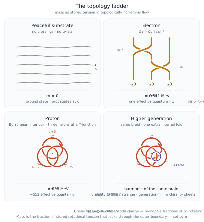
There is a second, independent description — the combinatorial view — that arrives at the same Standard Model spectrum by counting stable topologies of braided ribbons. Recent work by Bilson-Thompson, Lambek, and subsequent authors has shown that the fermionic content of the Standard Model’s SU(3)_c \times U(1)_{em} sector is reproduced exactly by the CPT-invariant elements of the braid group \mathcal{B}_3 acting on three ribbons, with twist operators generating electric charge and crossings generating chirality.4 The two pictures — hydrodynamic and combinatorial — are describing the same physical system from opposite ends, and the substrate framework provides what each one leaves implicit.
What the braid model sees
A helon is a ribbon with a half-integer twist (a quantized rotational tension along its length). Three helons braided together form a closed topological object whose properties are fully specified by two kinds of integer data:
- Crossings (\sigma_i^{\pm 1} in the braid group): how the three ribbons interlace. These map to elements of SL(2,\mathbb{Z}), which embeds inside SL(2,\mathbb{C}) — the double cover of the restricted Lorentz group. Crossings therefore encode chirality.
- Twists (T_i^{\pm 1} on each ribbon): integer units of rotational tension on each of the three strands. These map to weights on the U(1)_{em} axis of the weight lattice and encode electric charge.
Each Standard Model fermion has a specific braid word. For the left-handed electron: \sigma_1^{-1}\sigma_2 T_{123}^{-1} — one negative crossing between ribbons 1 and 2, one positive crossing between 2 and 3, and a negative twist on each of the three ribbons. Three unit twists sum to charge -1. The up-antiquark has \sigma_1\sigma_2^{-1}T_{12}^{-1} — opposite-sign crossings and only two twists, giving -2/3. The neutrino has only crossings, no twists — charge zero.
The mapping is not loose — it’s almost unreasonably tight
Line up the combinatorial elements of the braid model with the hydrodynamic elements of the substrate, and every row has a direct physical identification:
| Helon model element | Mathematical content | Substrate physical content |
|---|---|---|
| 3 ribbon strands | Basis of braid group \mathcal{B}_3 | 3 Y-junction branches of a vortex node (the Borromean interlocking of Proton Core) |
| Braid crossings \sigma_i^{\pm 1} | \mathcal{B}_3 \to SL(2,\mathbb{Z}) \hookrightarrow SL(2,\mathbb{C}) | Core flow winding through the junction; chirality of the co-rotating layer |
| Ribbon twists T_i^{\pm 1} | Integer weights on U(1)_{em} | Rotational tension pinched into each branch — the \pm 2/3, \pm 1/3 monopole fractions of a three-fold vortex junction |
| SU(3)_c \times U(1)_{em} weight lattice | Allowed fermion quantum numbers | Quantized boundary-matching conditions on the junction’s standing-wave pattern |
| CPT invariance of braids | Only SM fermions are CPT invariant | Dynamical stability of the vortex complex in the superfluid |
| The missing SU(2)_L | Not present in pure braid topology | Not a property of the particle — requires the chirally ordered substrate background (Higgs VEV) |
The last row is the decisive one. The preon paper explicitly notes that the helon model captures SU(3)_c \times U(1)_{em} but cannot account for the left-handedness of the weak interaction from pure topology alone, and speculates that additional strands beyond \mathcal{B}_3 may be required. The substrate framework says the same thing from the opposite direction: the weak asymmetry isn’t a topological property of the particle — it’s a strain on the particle’s outermost counter-rotating boundary when it moves through an already-chirally-ordered background field (Higgs Field). The Higgs VEV supplies what braid topology cannot. Both frameworks identify the same gap and point to the same physical object to fill it.
Why the double cover is free
The paper’s key mathematical move is the chain \mathcal{B}_3 \to SL(2,\mathbb{Z}) \hookrightarrow SL(2,\mathbb{C}) — the double cover of the restricted Lorentz group. This is the same double cover the Spin-Statistics chapter already identified: SO(3) is the symmetry of the co-rotating flow alone, SU(2) is the symmetry of the co-rotating + counter-rotating system together, with the 2:1 gear reduction between them (Higgs Field expands this in terms of the chirality field).
The counter-rotating boundary layer is literally the double cover in action. Each ribbon in a braid has a front and a back — a core and a boundary — and the phase relationship between them has double-cover topology by construction. The substrate framework provides the physical hardware for a mathematical mapping the preon paper has to take as a formal fact. The reason \mathcal{B}_3 lands inside SL(2,\mathbb{C}) is that each “ribbon” is secretly a co-rotating/counter-rotating pair — and that pair’s internal phase relationship is SU(2) all the way down.
CPT invariance = dynamical stability
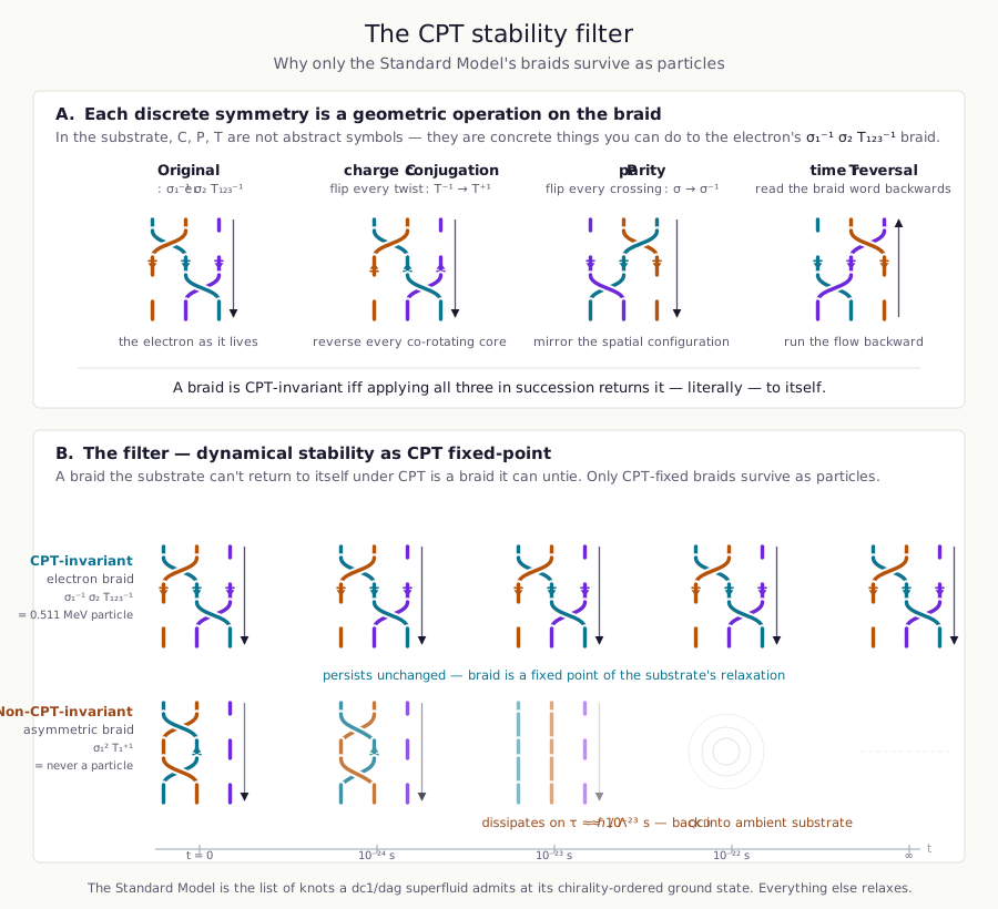
The most striking result of the preon work is that, out of the infinite tower of possible \mathcal{B}_3 braids, only the ones corresponding to known Standard Model fermions are CPT-invariant. No spurious particles. No unphysical states. This is wildly non-trivial from a pure representation-theoretic standpoint; the authors note that “braid diagrams of the helon model are precisely the only ones that happen to be CPT invariant” under their operational realization of the discrete symmetries.
In the substrate, this has a direct physical reading. Each discrete operation corresponds to a concrete flow-level symmetry of the vortex complex:
- C (charge conjugation): reverse the co-rotating core’s direction. Physically realizable in a superfluid — flow can reverse.
- P (parity): mirror the spatial configuration. Physically realizable — the dc1 medium is isotropic.
- T (time reversal): run the flow backward. Physically realizable — the substrate is dissipation-free (superfluid) at the level of its quasiparticle dynamics.
A braid that is invariant under all three operations is one that has found a true topological minimum against the substrate’s tendency to relax. A braid that fails any of them is a configuration the substrate can untie without crossing a barrier; it dissipates on superfluid timescales \sim 10^{-23} s and never gets counted as a particle. The Standard Model fermion spectrum is the list of knots that a dc1 superfluid admits as stable configurations at its chirality-ordered ground state. The preon paper proves this combinatorially; the substrate proves it dynamically; they have to agree because they are describing the same system.
Implications: the Yukawa hierarchy and the generation count
Two long-standing open problems look more tractable once the two frameworks are put side by side.
The Yukawa hierarchy. In the Standard Model, the coupling constants y_f that determine each fermion’s mass via m_f = y_f v/\sqrt{2} are 13+ free parameters with no structural explanation. The Higgs Field chapter argues that y_f is set by the effective boundary-interface area through which the fermion’s outermost counter-rotating layer couples to the background chirality field. The preon 5D weight-lattice coordinates give that interface area an integer label:
- 3 coordinates for twist charges on the three Y-junction branches (SU(3)_c)
- 1 coordinate for net chirality along the junction axis (U(1)_{em})
- 1 coordinate for outer-boundary handedness (the chirality state of the topmost counter-rotating layer)
Each weight-lattice point corresponds to a specific boundary architecture; the Yukawa coupling should be computable by projecting the boundary flow pattern onto the background chirality field’s eigenmodes. This turns Yukawa hierarchy from 13+ free parameters into a single cross-section calculation per weight-lattice point, using bulk substrate parameters already determined: \alpha_{mf} = 0.3008, m_\text{eff} = 1.70 MeV/c^2, r_\text{eff} = 150 fm.
The three-generation limit. The preon paper notes that higher fermion generations cannot fit inside \mathcal{B}_3 — they seem to require additional strands. The substrate framework says generations are radial excitations with additional internal boundary folds (Proton Core), and that the three chirality-coherent sheets of the 3D substrate lattice (Higgs Field — From Sheets to Stacking) are what make \mathcal{B}_3 appropriate in the first place. A generation-n fermion is a vortex complex that penetrates n chirality-coherent sheets. The three-generation limit is then the same calculation as the inter-sheet spacing d in the bridge equation — both determined by the chirality ordering thermodynamics at E_\text{core} \sim TeV. See Open Problems WIP-15 and WIP-Yukawa. Resolving one would resolve both.
This is also where the framework now makes the generations quantitative. The dedicated chapter Three Generations from One Turning Knot reads the three families as the three cube-roots-of-unity phases (\mathbb{Z}_3) of one three-fold junction; that \mathbb{Z}_3 structure, with the deviation amplitude fixed at the lattice’s pairing-\sqrt2, forces Koide’s charged-lepton relation Q=(\Sigma m)/(\Sigma\sqrt m)^2 = 2/3 to 9 ppm with no free parameter — and a single residual phase \delta=2/9 rad then lands the visibility ladder’s own rungs, m_\mu/m_e=206.77 and m_\tau/m_e=3477.5, to 0.001–0.007\%. So the diagonal m=\alpha_{mf}^\text{eff}m_\text{eff} below, which for most fermions only encodes each measured mass, becomes predictive in the charged-lepton sector: their relative visibilities are pinned by the three-fold geometry rather than read back.
The mass-topology synthesis
Putting the two descriptions together gives a single statement about what mass is:
A particle is a CPT-stable braid configuration of the substrate’s co-rotating/counter-rotating structure. Its rotational energy is the sum of twist tension (frozen into each ribbon) and crossing energy (frozen into the junction topology). The fraction of this energy that couples dissipatively to the surrounding substrate — set by \alpha_{mf} and by the topology’s effective interface area — is what a scale reads as rest mass.
The Standard Model asks: “What are the free parameters of this fermion’s mass?” and returns thirteen Yukawa couplings plus a VEV. The substrate asks: “What topological configuration is this?” and the answer is a braid word plus a visibility ratio — with the braid word determined by which CPT-stable knots the fluid admits, and the visibility ratio determined by the Weinberg angle’s dissipative fraction. Both pictures must be telling the same story because they describe the same physical object from opposite ends.
Boundary Layer Energy Budget
Boundary Energy Budget: The steady-state condition balances the kinetic energy input from substrate shear against the energy output carried away by emitted modons.
The boundary between two co-rotating regions stores energy in its counter-rotating layer. This section sketches the energy budget of such a boundary — a model that connects to photon emission rates and transition energies.
Steady-State Boundary
Consider two adjacent co-rotating vortex regions with velocity difference \Delta v across a boundary of thickness \delta and area A. The counter-rotating layer between them has density \rho_\text{cr}.
Energy stored in the boundary:
E_\text{boundary} = \tfrac{1}{2}\,\rho_\text{cr}\,(\Delta v)^2 \cdot A \cdot \delta
Energy input rate (shear from co-rotating regions driving the boundary):
\dot{W}_\text{in} = \tau_\text{shear} \cdot \Delta v \cdot A
In an inviscid superfluid, there is no viscous shear stress — instead, the “stress” comes from the momentum exchange of dc1 particles crossing the boundary:
\tau_\text{shear} = f_\text{cross} \cdot n_1 \cdot m_1 \cdot v_\text{flow} \cdot \Delta v
where f_\text{cross} is the probability per cell tick that a dc1 quantum crosses the boundary, and v_\text{flow} is the local substrate flow velocity at the boundary. For macroscopic (gravitational) boundaries, f_\text{cross} \approx 4.4 \times 10^{-31} (Gravity § Mathematical Form) and v_\text{flow} is at most the outer-rim speed v_\text{rot,outer} \approx 0.0025\,c. For inter-orbital-system boundaries at the atomic scale, v_\text{flow} and f_\text{cross} may differ — the same mechanism operates, but at a different scale.
Energy output rate (modons ejected from the boundary):
\dot{W}_\text{out} = \frac{N_\text{modon}}{\tau_\text{form}} \cdot E_\text{modon}
where N_\text{modon} is the number of modons that can form simultaneously in the boundary, \tau_\text{form} is the formation timescale, and E_\text{modon} is the energy per modon.
Steady-State Condition
\dot{W}_\text{in} = \dot{W}_\text{out}
f_\text{cross} \cdot n_1 \cdot m_1 \cdot v_\text{flow} \cdot \Delta v \cdot A = \frac{N_\text{modon}}{\tau_\text{form}} \cdot E_\text{modon}
Connection to Photon Emission
For an atomic transition where the boundary between orbital level N and N+1 reorganizes:
E_\text{photon} = E_\text{modon} = h\nu
\Delta v = v_{N+1} - v_N \quad\text{(velocity difference between orbital levels)}
The emission rate (photons per unit time from one boundary):
\Gamma_\text{emission} = \frac{N_\text{modon}}{\tau_\text{form}} = \frac{f_\text{cross} \cdot n_1 \cdot m_1 \cdot v_\text{flow} \cdot \Delta v \cdot A}{h\nu}
This is a testable prediction: given specific substrate parameters, this equation predicts the spontaneous emission rate for any atomic transition. Compare to the known Einstein A-coefficient:
A_{21} = \frac{\omega^3 \,|d_{12}|^2}{3\pi\,\varepsilon_0\,\hbar\,c^3}
These must agree. Matching them provides a constraint equation linking f_\text{cross}, n_1, m_1, and v_\text{flow} to known atomic physics.
Formation Timescale
The modon formation timescale should be roughly:
\tau_\text{form} \approx a / \Delta v \quad\text{(time for one vortex to roll up across the modon radius)}
For atomic transitions with \nu \sim 10^{15} Hz (visible light):
\tau_\text{form} \approx 1/\nu \approx 10^{-15} \;\text{s}
This is consistent with the timescale of electron orbital rearrangement during photon emission. The next chapter shows how the counter-rotating layer that stores this boundary energy is the physical origin of the quantum potential.
Footnotes
[R136] Aubert et al. (European Muon Collaboration), Phys. Lett. B 123, 275 (1983) — the discovery that the per-nucleon deep-inelastic structure function F_2^A/F_2^d deviates from unity in bound nucleons.↩︎
[R137] For g_A quenching resolved from first principles as coupling to correlations and two-body currents, Gysbers et al., Nature Physics 15, 428 (2019); the classic in-medium moment reduction traces to the modified meson cloud around a bound nucleon.↩︎
[R138] Hen, Miller, Piasetzky & Weinstein, Rev. Mod. Phys. 89, 045002 (2017) — reviews the linear correlation between the EMC-effect slope and the local binding (short-range-correlation) environment.↩︎
See Asselmeyer-Maluga et al., Preons, Braid Topology, and Representations of Fundamental Particles (arXiv preprint) for the explicit mapping between helon model braid states and the D_2 \oplus A_2 \oplus A_1 weight lattice. The combinatorial particle-centric view is complementary to the field-centric gauge theory view; the substrate framework provides the hydrodynamic hardware that realizes both.↩︎