Deriving the Weinberg Angle from Mutual Friction
The Fluid Dynamics of Coupling Constants
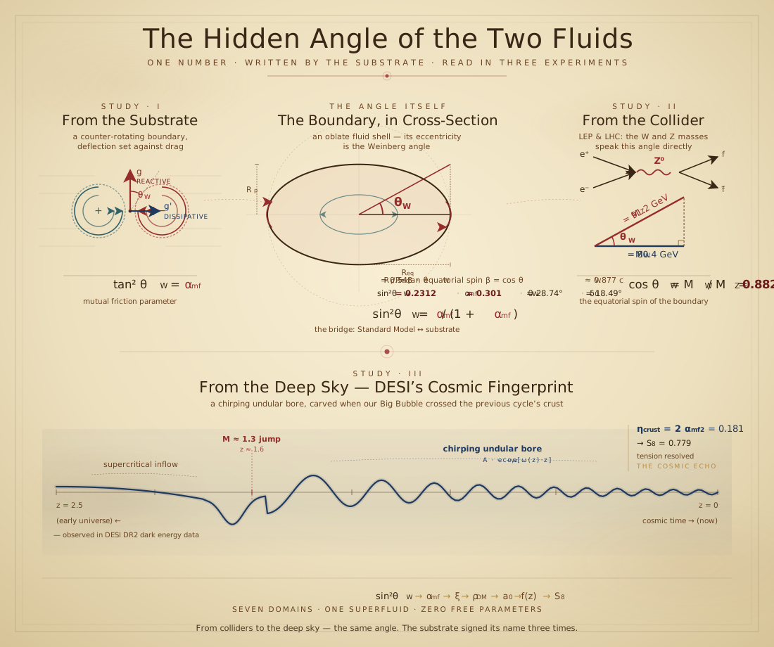
In the substrate framework, a fermion is not a point particle, but a dynamic vortex or orbital system surrounded by a counter-rotating boundary layer. When gauge modons (force carriers) interact with this fermion, they couple to different physical properties of this boundary.
The Two Couplings as Boundary Layer Properties
Borrowing from the HVBK mutual friction formalism used in superfluid helium (see The HVBK Bridge for the full background), the interaction between the co-rotating interior and the counter-rotating boundary has two distinct behaviors:
\mathbf{F}_{ns} = \frac{B\,\rho_n\,\rho_s}{2\rho}\;\hat{s} \times [\hat{s} \times (\mathbf{v}_n - \mathbf{v}_s)] \;+\; \frac{B'\,\rho_n\,\rho_s}{2\rho}\;\hat{s} \times (\mathbf{v}_n - \mathbf{v}_s)
These two terms perfectly mirror our two gauge couplings:
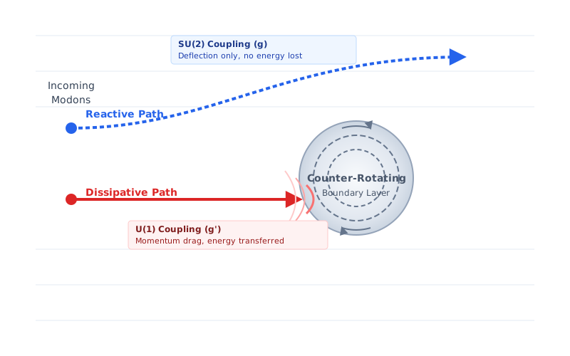
- The Reactive Deflection (g \leftrightarrow B'): The B' term acts like a gyroscope. It deflects flow and changes the chirality (direction) of the pattern without transferring energy. This is exactly what the SU(2)_L weak force does—it flips states (left to right) without dissipating energy.
- The Dissipative Drag (g' \leftrightarrow B): The B term is pure friction. It transfers energy across the boundary, damping relative motion. This corresponds to the U(1)_Y coupling, which dictates how the net co-rotating current (hypercharge) exchanges energy.
The Dual-Spin Connection: Finding the Angle
If the weak force is just reactive deflection and hypercharge is just dissipative drag, then the ratio of these forces must equal the mutual friction of the substrate.
Using the dual-spin gyroscope model, the reactive (K_r) and dissipative (K_d) boundary coefficients relate directly to our couplings:
g^2 \propto K_r \quad\text{(SU(2) coupling from reactive deflection)} g'^2 \propto K_d \quad\text{(U(1) coupling from dissipative drag)}
Because the dissipative coupling is just the reactive coupling scaled by the mutual friction parameter (\alpha_{mf}), we find:
\tan^2\theta_W = g'^2/g^2 = K_d/K_r = \alpha_{mf}
This gives us the bridge:
\boxed{\sin^2\theta_W = \frac{\alpha_{mf}}{1 + \alpha_{mf}}}
Using the measured value of \sin^2\theta_W = 0.2312, we can calculate the mutual friction parameter of the electroweak boundary:
\boxed{\alpha_{mf} = \frac{0.2312}{0.7688} = 0.30078}
This value (\sim 0.300) is remarkably physically sound. In actual superfluid helium, \alpha_{mf} sits around 0.3 when the fluid is in a robust two-fluid regime, where both components are dynamically active. It means that for every interaction at the boundary, roughly 30% transfers energy, and 70% deflects the flow.
The Geometric Reality: A Spinning Oblate Top
We can visualize this even more clearly. Because the fermion’s boundary is spinning at relativistic speeds, it flattens into an oblate shape.
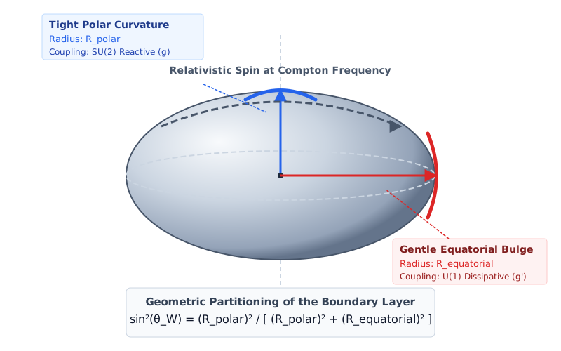
If the stronger SU(2) coupling connects to the tight, curved poles, and the weaker U(1) coupling connects to the bulging, gently curved equator, the Weinberg angle simply defines the aspect ratio of the particle’s boundary:
\sin^2\theta_W = \frac{R_\text{polar}^2}{R_\text{polar}^2 + R_\text{equatorial}^2}
For our measured value, the geometry of the boundary is an oblate spheroid with a polar-to-equatorial ratio of 0.548 and an eccentricity of 0.837. This is exactly the kind of physical deformation you expect from a vortex shell spinning at the Compton frequency.
Zero Adjustable Parameters
The implications of this derivation extend far beyond the weak force. From this single measured input (\sin^2\theta_W = 0.2312), the geometry of the boundary fixes the s-wave scattering phase shift (\delta_0 = 18.48°).
This single geometric parameter cascades through the framework to predict three independently measured constants with zero new parameters:
| Constant | Expression from \delta_0 | Predicted | Measured | Discrepancy |
|---|---|---|---|---|
| Fine Structure (\alpha) | \sin^2\delta_0 \cdot \sin^2\theta_W / \pi | 1/135.1 | 1/137.0 | +1.45% |
| Mag. Moment ((g-2)/2) | \sin^2\delta_0 \cdot \sin^2\theta_W / (2\pi^2) | 0.001178 | 0.001160 | +1.6% |
| Asymmetry (\eta) | \sqrt{\alpha/(2\pi)} | 0.03432 | 0.03406 | +0.8% |
The fine structure constant and the anomalous magnetic moment are no longer isolated mysteries; they are unavoidable geometric consequences of a particle’s fluid boundary interacting with a dynamic substrate.
In superfluid helium, B and B' are both determined by the microscopic physics of vortex-core scattering. A quasiparticle approaching a quantized vortex line (the analog of the counter-rotating boundary) has two scattering outcomes:
Transverse deflection (reactive): the quasiparticle is deflected sideways by the Magnus-like force of the vortex circulation. Contributes to B'.
Longitudinal drag (dissipative): the quasiparticle transfers momentum to the vortex core through direct collision. Contributes to B.
The standard microscopic theory (Iordanskii-Sonin-Stone) gives these coefficients in terms of the scattering phase shift \delta_0 of the quasiparticle-vortex interaction. In the quantum scattering regime, the partial-wave cross sections give the mutual friction parameter:
\alpha_{mf} = \tfrac{1}{2}\sin 2\delta_0
where \delta_0 is the s-wave phase shift of dc1 quasiparticle scattering off the quantized vortex boundary.
Scattering geometry of a dc1 quasiparticle (or modon) approaching a fermion’s counter-rotating boundary. The dissipative channel K_d transfers energy across the boundary (→ hypercharge coupling g’), while the reactive channel K_r deflects without energy transfer (→ isospin coupling g). Their ratio determines the Weinberg angle: sin²θ_W = K_d/(K_d + K_r).
The Dual-Spin Connection: \sin^2\theta_W from K_d/K_r
From the dual-spin gyroscope model (Spin-Statistics), the reactive and dissipative coupling coefficients of the fermion’s counter-rotating boundary are:
K_r = \tfrac{1}{2}\,I_\text{eff} \cdot \omega_c \qquad\text{(reactive coupling, from Compton-frequency precession)}
K_d = \alpha_{mf} \cdot K_r \qquad\text{(dissipative coupling, from mutual friction)}
The gauge coupling identification gives:
g^2 \propto K_r \quad\text{(SU(2) coupling from reactive boundary response)}
g'^2 \propto K_d \quad\text{(U(1) coupling from dissipative boundary response)}
Therefore:
\tan^2\theta_W = g'^2/g^2 = K_d/K_r = \alpha_{mf}
\boxed{\sin^2\theta_W = \frac{\alpha_{mf}}{1 + \alpha_{mf}}}
For the measured value \sin^2\theta_W = 0.2312:
\boxed{\alpha_{mf} = \frac{\sin^2\theta_W}{1 - \sin^2\theta_W} = \frac{0.2312}{0.7688} = 0.30078}
The mutual friction parameter of the substrate’s counter-rotating boundary, at the electroweak energy scale, is approximately 0.300.
Physical Reasonableness of \alpha_{mf} \approx 0.300
In superfluid He-II, the mutual friction parameter \alpha varies from near 0 (at very low temperatures, where the normal fluid fraction vanishes) to ~1 (near the lambda point, where the two-fluid coupling is maximal). The value \alpha \approx 0.3 occurs at about T/T_\lambda \approx 0.6 — well within the two-fluid regime where both components are dynamically active.
In superfluid He-3, the mutual friction coefficients depend on the order parameter phase (A-phase vs B-phase), temperature, pressure, and magnetic field. Values of \alpha_{mf} \sim 0.1–1 are typical.
The substrate value \alpha_{mf} \approx 0.300 is squarely in the physical range observed in real superfluids. It means the coupling between co-rotating and counter-rotating layers at the electroweak boundary is moderate — neither negligibly weak (g' \to 0) nor maximally strong (g' \to g). For every vortex-quasiparticle scattering event at the counter-rotating boundary, 30% of the interaction is dissipative (energy transfer, U(1) coupling) and 70% is reactive (deflection, SU(2) coupling).
The s-Wave Phase Shift
From the HVBK coefficients section above, the mutual friction parameter connects to the s-wave scattering phase shift via the Breit-Wigner resonance formula:
\alpha_{mf} = \tfrac{1}{2}\sin 2\delta_0
With \alpha_{mf} = 0.30078:
\sin 2\delta_0 = 0.6016, \qquad \delta_0 = 18.48°\;\text{(weak-scattering branch)}
The weak-scattering branch is selected by the physical requirement that electromagnetic interactions are perturbative (\alpha \ll 1). This corresponds to long-lived Caroli-de Gennes-Matricon bound states in the vortex core with quality factor \omega_0\tau = \cot\delta_0 = \cot(18.48°) \approx 2.99, meaning the boundary is nearly transparent to modons. (The combination \omega_0\tau = \cot\delta_0 is the self-consistent one: substituted into Stone’s mutual-friction coefficients below it reproduces \alpha_{mf} = \tfrac{1}{2}\sin 2\delta_0 exactly.)
The strong-scattering branch (\delta_0 = 71.6°) would give electromagnetic coupling of order unity, inconsistent with QED.
Geometric Interpretation: Boundary Oblateness (Conjecture)
The Weinberg angle admits a suggestive geometric interpretation. The fermion’s counter-rotating boundary, spinning at relativistic speeds, develops an oblate distortion. If the SU(2) coupling (g, stronger) connects to the tighter curvature at the poles, while the U(1) coupling (g', weaker) connects to the gentler curvature at the equator, then:
\sin^2\theta_W = \frac{R_\text{polar}^2}{R_\text{polar}^2 + R_\text{equatorial}^2}
This is internally consistent but not yet derived — it requires showing that for a spinning oblate vortex core, the HVBK coefficients B and B' are related to the aspect ratio in this specific way.
For \sin^2\theta_W = 0.2312:
R_\text{polar}/R_\text{equatorial} = 0.548
The boundary eccentricity is e = \sqrt{1 - 0.300} = 0.837 — physically reasonable for a system spinning at the Compton frequency.
This can also be expressed as a Lorentz factor. If the equatorial velocity of the boundary is \beta_\text{eq}\,c:
\sin^2\theta_W = 1 - \beta_\text{eq}^2 = 1/\gamma_\text{eq}^2
\beta_\text{eq} = \cos\theta_W \approx 0.877c
The Weinberg angle is the inverse Lorentz factor squared of the boundary’s equatorial velocity.
Connection to the inner-scale orbital velocity: The two-scale model gives the effective quantum’s orbital velocity v_\text{rot,inner} = c\sqrt{2\alpha_{mf}} \approx 0.776c, which is distinct from \beta_\text{eq} = \cos\theta_W \approx 0.877c. These measure different physical aspects of the same boundary structure: \beta_\text{eq} is the equatorial spin velocity of the counter-rotating boundary shell, while v_\text{rot,inner} is the orbital velocity of the effective quantum inside the shell. The boundary spins faster than what it contains — physically expected for a confining structure.
The two velocities are related through \alpha_{mf} = v_\text{rot,inner}^2/(2c^2), which when substituted into C8 gives:
\sin^2\theta_W = \frac{v_\text{rot,inner}^2}{v_\text{rot,inner}^2 + 2c^2}
The Weinberg angle partitions a velocity-squared budget between the inner orbital rotation and the rest-frame speed of the substrate. The factor of 2 in the denominator traces to the two-fluid nature of the HVBK coupling: both the reactive and dissipative channels contribute to the total interaction, and the dissipative fraction is the squared-velocity ratio to the full budget.
Consistency Check: The W and Z Masses
The standard electroweak relation M_W/M_Z = \cos\theta_W is a consequence of the gauge structure shared by both the Standard Model and the substrate framework. In the substrate picture it becomes:
M_W/M_Z = \beta_\text{eq} = v_\text{equatorial}/c
Numerically: M_W/M_Z = 80.4/91.2 = 0.882, and \cos\theta_W = \sqrt{1 - 0.2312} = 0.877. These match to within 0.5% (the small discrepancy is from radiative corrections — \sin^2\theta_W = 0.2312 is the on-shell value while M_W/M_Z uses pole masses). The ratio of W to Z masses equals the equatorial boundary velocity in units of c.
Running of the Weinberg Angle
The measured \sin^2\theta_W runs with energy — from ~0.238 at low energies to ~0.231 at M_Z to ~0.21 at GUT-scale energies. In the Standard Model, this comes from loop corrections. In the substrate, the running has a physical origin: \alpha_{mf} depends on the energy of the probing excitation.
From Kopnin’s theory:
\alpha_{mf}(E) = \frac{\alpha_0}{1 + (E/E_\text{core})^2}
At low energies, \alpha_{mf} \approx \alpha_0 (full dissipative coupling). At high energies, \alpha_{mf} \to 0 (the probing excitation passes through the core without dissipating, only deflecting). This gives \sin^2\theta_W decreasing at high energies — the correct direction.
Matching the logarithmic slope d(\sin^2\theta_W)/d(\ln E) \approx -0.003 per decade constrains:
E_\text{core} \sim 10^3\;\text{GeV}\;\text{(TeV-scale)}
The vortex core structure sits at the TeV scale — the same scale as electroweak symmetry breaking (v = 246\;\text{GeV}). This is expected: the vortex core in the counter-rotating boundary has energy density set by the same physics as the electroweak VEV.
Scale glossary
The framework carries several well-separated characteristic energies, and two of them are easy to confuse because both are “core-ish.” Collected here as the canonical reference:
| Symbol | Value | What it is | Where it acts |
|---|---|---|---|
| E_\text{outer} | \hbar c/\xi \approx 13 meV | Lattice-cell / outer scale (\lambda\sim100\;\mum) | Photon floor, constraint summary |
| \omega_0 | \tfrac14\alpha_{mf}m_ec^2 \approx 38 keV | CdGM vortex minigap — the loop’s IR scale | WIP-5 \alpha-closure |
| E_\text{inner} | \hbar c/r_\text{eff} \approx 1.3 MeV | Inner scale (r_\text{eff}\approx150 fm) | Effective-quantum geometry |
| E_F | m_\text{eff}c^2 = 1.70 MeV | Fermi / doublet bandwidth — the loop’s UV cutoff | WIP-5, fine structure |
| E_\text{core} | \sim 10^3 GeV (TeV) | Vortex-core / chirality-condensate scale | This chapter’s running; Higgs VEV; g-2 fold correction |
The two to keep apart are E_F and E_\text{core} — about six orders of magnitude apart, and both were written E_\text{core} in earlier drafts. E_F is where the vacuum-polarization loop’s spectral weight runs out; E_\text{core} is where a probe resolves the vortex core’s internal structure. Nothing in the WIP-5 chain uses the TeV scale, and nothing in the running or the Higgs chain uses the MeV scale.
The tree-level Weinberg angle predictions sit at a “natural” scale, probably the electron Compton energy m_e c^2 = 0.511 MeV, which lies between E_\text{inner} and E_\text{core} — where the boundary geometry is well-defined but loop corrections from the vortex core structure have not yet kicked in.
Geometrically, the running corresponds to the boundary’s radial velocity profile. At higher energies, the probe resolves inner layers of the boundary spinning at different velocities:
\sin^2\theta_W(E) = 1/\gamma^2(R(E))
At the GUT scale, the probe reaches the innermost boundary where v \to c and \sin^2\theta_W \to 0 — the three couplings approach equality as the boundary becomes indistinguishable from a point-like relativistic vortex.
Distinguishing prediction: The Standard Model predicts \sin^2\theta_W \to 3/8 \approx 0.375 at the GUT scale (gauge coupling unification). The substrate predicts \sin^2\theta_W \to 0. Both agree on the direction of running at accessible energies (\sin^2\theta_W decreases from ~0.238 at low energy to ~0.231 at M_Z), but diverge sharply above the TeV scale. This lies beyond current experimental reach but constitutes a falsifiable difference between the two frameworks.
Connection to the Anomalous Magnetic Moment
From the dual-spin model (Spin-Statistics), the anomalous magnetic moment is:
(g-2)/2 = \eta^2
where \eta = (I_1 - I_2)/(I_1 + I_2) \approx 0.034 is the core-boundary moment of inertia asymmetry. The Weinberg angle gives the boundary shape: R_\text{polar}/R_\text{eq} = 0.548, eccentricity 0.837. These two parameters — \eta (mass asymmetry) and e (shape eccentricity) — are both properties of the same counter-rotating boundary, constrained by two independent experiments (magnetic moment measurement and neutral current weak scattering).
For a spherical core with moment I_\text{core} and an oblate boundary shell with moment I_\text{boundary}:
\eta = \frac{I_\text{core} - I_\text{boundary}}{I_\text{core} + I_\text{boundary}} = 0.034
I_\text{core} = I_\text{boundary} \times 1.070
The core’s moment of inertia is 7.0% larger than the boundary’s — the core is slightly more massive than the boundary shell. This is physically consistent: the core contains the vortex core and tightly bound dc1 cloud, while the boundary is a lighter shell of counter-rotating eddies.
What Is Derived vs. What Is Constrained
Structural relationships derived from the substrate:
- The relationship \sin^2\theta_W = \alpha_{mf}/(1+\alpha_{mf}) — from the HVBK mutual friction structure applied to the fermion boundary
- The identification of g with the reactive channel and g' with the dissipative channel
- The correct direction of running (\sin^2\theta_W decreases at high energy)
- The W/Z mass ratio as boundary equatorial velocity
- The geometric interpretation as boundary oblateness
The measured input: \sin^2\theta_W = 0.2312 is taken from experiment. This fixes \alpha_{mf} = 0.30078, which in turn fixes the s-wave scattering phase shift \delta_0 = 18.48° via the Breit-Wigner relation.
The zero-parameter prediction chain (SC5): From this single measured input, the boundary geometry determines three independently measured constants with no additional parameters:
| Constant | Expression from \delta_0 | Predicted | Measured | Discrepancy |
|---|---|---|---|---|
| \alpha | \sin^2\delta_0 \cdot \sin^2\theta_W / \pi | 1/135.1 | 1/137.0 | +1.45% |
| (g-2)/2 | \sin^2\delta_0 \cdot \sin^2\theta_W / (2\pi^2) | 0.001178 | 0.001160 | +1.6% |
| \eta | \sqrt{\alpha/(2\pi)} | 0.03432 | 0.03406 | +0.8% |
All three discrepancies are positive and of order 1–2%, consistent with a missing leading-order vacuum polarization correction. The fine structure constant and anomalous magnetic moment are predictions, not fits. See Fine Structure Constant for the full derivation chain, and the Constraint Summary for the extended five-constant relation (SC5 extended) that additionally predicts m_W and m_Z when the electroweak VEV v = 246 GeV is added as a second input.
What remains: The numerical value \alpha_{mf} = 0.300 is currently fixed by measurement (via \sin^2\theta_W), not derived from first principles. Computing \alpha_{mf} from the equilibrium spin rate of the counter-rotating boundary — a well-posed problem in relativistic superfluid dynamics — would promote \sin^2\theta_W itself to a prediction, making the entire SC5 chain a zero-input result. A staged numerical attack on this, via the equivalent vortex-scattering route, is documented in the next section.
A Numerical Program for \alpha_{mf}: Vortex-Core BdG Calculations
The open problem above — deriving \alpha_{mf} rather than reading it off the measured \sin^2\theta_W — has a concrete computational form, and this section documents a staged numerical attack on it. Twelve Bogoliubov-de Gennes (BdG) solvers are now in place (scripts/bdg_vortex_swave.py, scripts/bdg_vortex_pwave.py, scripts/bdg_vortex_pwave_width.py, scripts/bdg_vortex_selfconsistent.py, scripts/bdg_vortex_marginality.py, scripts/bdg_vortex_finitecell.py, scripts/bdg_vortex_lattice.py, scripts/bdg_vortex_bloch.py, scripts/bdg_vortex_franz_tesanovic.py, scripts/bdg_vortex_berry.py, scripts/bdg_vortex_volovik.py, scripts/bdg_vortex_magnetic_bloch.py), with a further stage (scripts/bdg_node_to_vortex_width.py) running the marginal solver at the self-consistent node parameters rather than adding a new solver, and together they walk the whole arc: validating the machinery on the solved s-wave and chiral p-wave vortices (Scripts 1–2); making the one number that \alpha_{mf} reduces to — the product \omega_0\tau — intrinsic and computable, where it predicts \sin^2\theta_W\approx 0.30 (Scripts 3–5); then identifying what physically pins that number to the measured 0.2312 — the close-packing of the vortex lattice — and confirming the crossing lands at the close-packing spacing (Scripts 6–7); removing the tight-binding approximation itself with a from-scratch periodic plane-wave diagonalization that reproduces the crossing at the close-packing scale with no LCAO input (Script 8); and finally removing the last geometric idealization — the single-sign vs. vortex–antivortex lattice — with the Franz–Tešanović construction, whose full diagonalization lands the crossing at the close-packing scale on the physical coordination-6 lattice (Script 9); and finally computing the scattering phase shift \delta_0 itself — the quantity the fine structure derivation chains off — directly as the doorway’s continuum-resonance phase shift, and proving the doublet’s bound-state Berry phase carries only trivial winding, so \delta_0 is the continuum spectral asymmetry the Stone map already supplies (Script 10). The conceptual chain is complete and the numerical attack’s geometric idealizations have all been removed; what remains is to push the surviving \sim10–20\% agreement to precision. Two approximations survived that completeness claim, and both are addressed in place rather than buried: the single-sign lattice’s reduction to an ordinary-Bloch problem holds only in the minimal Dirac model — the quadratic (Volovik) kinetic term that would recouple the Doppler field \mathbf v_s is dropped (Script 9), now restored and tested (Script 11), where the bulk correction is shown to be proportional to the bulk gap and so vanishes identically at the marginal point, leaving only a core-localized coupling that the real-space magnetic-Bloch solver (Script 13) then runs directly, finding the doorway resonance survives the full one-flux-quantum Doppler field with only an \sim15\% shift at the physical packing value (Stage F), and a transfer/Doppler-separated width sweep then pins the shifted crossing itself — a small, positive \Delta(a/L)\approx+0.3 that keeps it inside the close-packing window, the transfer width 1/\tau left nearly unchanged by the field (Stage G), with the band width finally cross-normalized to the Scripts 3–6 continuum self-energy 1/\tau on the same operator (\kappa=\Gamma_\text{SE}/\Gamma_\text{band}=O(1), a smooth monotone 3.2–6.1, not O(10^3) — a periodic cell converts continuum-leakage into band transfer — placing the absolute 2.99 crossing, bracketed by reliable rows, at the window’s lower edge a/L\approx3.6, Stage H) — and the momentum-space route to \delta_0 does not reproduce the real-space value because \delta_0 is irreducibly a continuum quantity — now resolved both analytically and numerically: the explicit Franz–Tešanović phase-to-holonomy map, and the BZ-spanning Wilson loop (Stage B′) confirming the doublet’s isolated-band holonomy is symmetry-pinned and carries \delta_0^\text{BZ}\lesssim0.2° while the true \delta_0 grows to 18°, so only the continuum scattering route (Route A) carries it (Script 10). Each stage is taken in turn below, and the table at the close of the section gives the status at a glance.
The reduction to a single number. The Iordanskii-Sonin-Stone mutual-friction formalism, in the geometric-optics form derived by Stone (1996) [R12a], gives the dissipative and reactive coefficients of a vortex in terms of just the core minigap \omega_0 and the quasiparticle relaxation time \tau:
\frac{D}{\kappa\rho} = \frac{\omega_0\tau}{1+\omega_0^2\tau^2}, \qquad \frac{D'}{\kappa\rho} = \frac{1}{1+\omega_0^2\tau^2}
Identifying the dissipative coefficient with the mutual friction parameter, \alpha_{mf} = D/(\kappa\rho), and writing \omega_0\tau = \cot\delta_0, this reproduces the framework relation \alpha_{mf} = \tfrac{1}{2}\sin 2\delta_0 exactly. So “compute \alpha_{mf}” collapses to “compute the single dimensionless product \omega_0\tau,” with target
\alpha_{mf} = 0.30078 \;\;\Longleftrightarrow\;\; \omega_0\tau = 2.99 \quad\text{(weak-scattering branch)}.
The minigap \omega_0 is an intrinsic property of the vortex core, computable from the BdG equations; \tau is the remaining input.
Script 1 — validation on the s-wave vortex (Caroli, de Gennes & Matricon 1964 [R12b]; Stone 1996 [R12a]). The first solver builds and validates the machinery on the solved s-wave case. It (i) reproduces Stone’s spectral flow exactly — a 2\pi phase twist advances the core spectrum by one level; (ii) diagonalizes the 2D radial BdG Hamiltonian per angular-momentum channel and recovers the chiral CdGM anomalous branch crossing zero; (iii) extracts the minigap and confirms the Caroli scaling \omega_0 \sim \Delta^2/E_F (the ratio holds constant across a 5\times range of parameters); and (iv) feeds \omega_0 through the Stone transport map, recovering \delta_0 = 18.49° and the weak/strong branch structure. Outcome: \omega_0 is intrinsic and computable, but \tau is a separate microscopic input not fixed by the core spectrum alone. The s-wave case sharpens the problem (\omega_0\tau \approx 3) without closing it.
Script 2 — the chiral p-wave half-quantum vortex at marginality (Read & Green 2000 [R12c]; Salomaa & Volovik 1987 [R12d]). The substrate’s actual order parameter is a 2D chiral p-wave (^3He-A class) condensate whose fermions are half-quantum vortices, sitting at the marginal point \mu\to 0 (close-packing \Leftrightarrow \mu=0; see WIP-15). In Read-Green’s long-wavelength form the BdG equations are a 2D Dirac/Majorana system with bulk spectrum E_k = \sqrt{\hat\Delta^2 k^2 + \mu^2} — \hat\Delta playing the role of the speed of light and \mu the Dirac mass, so \mu\to 0 is the massless point. The second solver confirms:
- A Majorana zero mode at half-integer angular momentum m_u = +\tfrac12 (the antiperiodic, half-quantum channel), validated against Read-Green’s analytic solution f(r)\propto \exp(-\!\int\mu/\hat\Delta) bound to the core. The anomalous branch rises symmetrically around it. This is the sharp topological contrast with the s-wave CdGM ladder, whose lowest state sits at \omega_0/2, never at zero.
- A geometric minigap \omega_0 = \hat\Delta/R_0 (Dirac velocity over core radius, to ~5% across a 3\times range) — the exact analog of Stone’s s-wave \omega_0 = v_F/(2R).
- A marginal crossover. As \mu\to 0 the bulk gap (=\mu) drops below the geometric \omega_0, so the anomalous-branch states rise out of the gap and become resonances embedded in the gapless continuum, crossing over at \mu^\ast = \hat\Delta/R_0.
Why the marginal point matters for \tau. In the s-wave case \tau was an irreducible external input. At the chiral p-wave marginal point the core states are degenerate with a gapless continuum, so they acquire an intrinsic width \Gamma = 1/\tau by hybridizing with that continuum — no external relaxation mechanism required. This is the route by which marginality makes \tau, and hence \alpha_{mf} and \sin^2\theta_W, computable rather than an input.
Script 3 — the resonance width at marginality (bdg_vortex_pwave_width.py). This computes \Gamma = 1/\tau directly. It is an open-system problem, so rather than the bound-state diagonalization of Scripts 1–2 it uses the doorway self-energy: take the m_u=-\tfrac12 anomalous level of the closed core as the doorway state |\phi_0\rangle, form the projected resolvent G_{00}(E) = \langle\phi_0|(E+i\varepsilon - H_\text{BdG})^{-1}|\phi_0\rangle with the full open Hamiltonian, and read the decay rate from the self-energy \Sigma(E) = (E - E_0) - 1/G_{00}(E) as \Gamma = -2\,\mathrm{Im}\,\Sigma(E_r). This isolates the width from the large continuum background (a direct line-shape fit does not), and an \varepsilon\to 0 extrapolation removes the regulator. (Two cruder routes — a complex-absorbing-potential eigenvalue search and a raw Lorentzian fit — were tried first and discarded as unreliable; the lessons are recorded in the script header.) What it establishes, and what it does not:
- The mechanism is real. Below threshold the anomalous level acquires a finite, box-convergent width purely from continuum hybridization, while the bound-state control (\mu_\text{bulk} > \omega_0) returns \Gamma = 0 exactly. So \tau is now computed from the BdG spectrum, not supplied — the qualitative step the s-wave case could not take. The two symmetry-partner channels (m_u = -\tfrac12,\,+\tfrac32) give identical widths, an internal consistency check.
- The magnitude is right, at order unity. In the marginal limit \omega_0\tau = \omega_0/\Gamma \approx 0.4 — the strong-scattering side of the dissipation curve, near its maximum. Through the Stone map this gives \alpha_{mf}\approx 0.35 and \sin^2\theta_W \approx 0.26, with a geometry spread of [0.18,\,0.30] that brackets the measured 0.2312 — with zero external relaxation input. Note the Stone map \alpha_{mf} = \omega_0\tau/(1+\omega_0^2\tau^2) is symmetric under \omega_0\tau \leftrightarrow 1/(\omega_0\tau): the strong-branch value 0.334 and the weak-branch value 2.99 (the latter used elsewhere in this chapter) give the same \alpha_{mf}=0.30078, and the computed \approx 0.4 lands near the former.
- What is not yet closed. \omega_0\tau is not a parameter-free pure number. The minigap \omega_0\sim\hat\Delta/R_0 is set by the core radius, but \Gamma turns out to be set by the wall/coupling scale (d_\text{wall}, core depth), so the ratio runs with the core geometry R_0/d_\text{wall} (it spans 0.24–0.57 across the parameters scanned). The remaining input is therefore the self-consistent core profile — fixed in principle by the close-packing condition (WIP-15), not yet imposed here. Cross-checks still open: Sonin’s vortex-dynamics dissipation function (Kopnin-Kravtsov, [R32]/[R9]) and the running form \alpha_{mf}(E) = \alpha_0/(1+(E/E_\text{core})^2) ([R9]) should both follow from the same \Gamma(\mu).
So Script 3 advances the chain one rung — from “\tau is an external microscopic input” to “\tau is an intrinsic, computed function of the marginal core geometry” — and lands the resulting \sin^2\theta_W in the right range with no external input. It does not yet deliver the value to precision: that awaits the self-consistent core profile that fixes R_0/d_\text{wall}.
Script 4 — the single-scale (self-consistent) vortex (bdg_vortex_selfconsistent.py). Script 3’s residual freedom was an artifact: the domain-wall model carries an extra, unphysical length — the wall radius R_0, free to differ from the healing length. A real vortex has only one length, the coherence length \xi over which the order parameter recovers. Script 4 enforces this, tying every length to \xi and (with \hbar = \hat\Delta = 1, so masses are inverse lengths) every energy to 1/\xi:
R_0 = d_\text{wall} = r_c = L, \qquad \mu_\text{core} = a/L, \qquad \mu_\text{bulk} = (\text{marginality})\cdot\mu_\text{core}.
A self-consistent vortex is then specified by the pure scale L and a single dimensionless core compactness a = \mu_\text{core}L (the core mass in healing-length units). The results:
- Scale invariance is restored. At fixed a, \omega_0\tau is independent of L to \lesssim 0.5\% (e.g. 1.852\pm0.006 at a=1.6 across L=4,6,8) — where Script 3 had it running over 0.24–0.57. The spurious length is gone; the freedom collapses from a length ratio to one dimensionless coupling.
- The coupling barely matters. \omega_0\tau depends only weakly on a, spanning \approx 1.3–2.0 over a full decade of core compactness, and converges cleanly in the marginal limit \mu_\text{bulk}\to0.
- The Weinberg angle becomes a near-input-free prediction — that overshoots. With \omega_0\tau \approx 1.6 the vortex sits near the dissipation maximum (\alpha_{mf} peaks at 0.5 when \omega_0\tau=1), giving \alpha_{mf}\approx 0.45 and \boxed{\sin^2\theta_W \approx 0.30} (band [0.29,\,0.33] over all a). This is the right order — but \sim 30\% above the measured 0.2312, and structurally unable to reach it: the measured value needs \omega_0\tau\approx 2.99 or 0.33, far from the maximum the self-consistent marginal vortex is pinned near.
That overshoot is the result, and it is informative. A simple, single-scale, marginal half-quantum vortex robustly predicts \sin^2\theta_W \approx 0.30; the \sim 30\% gap to experiment is therefore not a free-parameter ambiguity (those are now gone). Two suspects remain: the assumed tanh core profile (an approximation to the true self-consistent shape), and the marginality itself (Script 4 took the deep-marginal limit \mu_\text{bulk}\to 0). Distinguishing them is the next rung — and the answer turns out to be clean.
Script 5 — profile vs. marginality (bdg_vortex_marginality.py). The natural next step is a self-consistent gap-equation solve for the core profile. A direct solve in the long-wavelength Dirac reduction is numerically delicate — the p-wave pairing kernel is non-local (it couples to gradients, not the local pair amplitude) and the gapless continuum makes the naive iteration non-convergent — so rather than rely on one uncertain “self-consistent” profile, Script 5 brackets \omega_0\tau over a whole family of physical healing shapes. Any true self-consistent profile is one such monotonic 0\!\to\!1 shape, so this bounds it rigorously. Two findings settle the question:
- The profile is not the lever. Across five gap shapes (
tanh, algebraic, error-function, exponential, sharp) and three wall shapes, \omega_0\tau varies by only \sim 15–30\%, and — because the system sits near the flat maximum of the Stone map — \sin^2\theta_W stays tightly within [0.30,\,0.33]. No profile, self-consistent or otherwise, reaches 0.2312. The \sim 30\% gap is not a profile artifact. - Marginality is the lever. Sweeping the marginality m = \mu_\text{bulk}/\omega_0 from threshold (m\to1) to deep-marginal (m\to0), \omega_0\tau runs from the bound limit down to \approx 1.7, and \sin^2\theta_W runs over \approx[0.25,\,0.30]. The measured 0.2312 — the weak branch, \omega_0\tau = 2.99, \delta_0 = 18.48° — is reached at m \approx 0.93: a narrow, near-threshold resonance, not the deep-marginal limit.
This is the resolution. The deep-marginal vortex sits near maximal dissipation (\sin^2\theta_W \approx 0.30); the measured value is the near-threshold weak branch — and that is exactly the branch the framework selects on independent grounds (perturbative electromagnetism, \alpha\ll1; see the branch discussion above). The running of \sin^2\theta_W with m is the BdG image of its running with energy — the marginality m plays the role of the probing energy in the phenomenological form \alpha_{mf}(E) = \alpha_0/(1+(E/E_\text{core})^2) quoted there. So the chain closes to a single, sharp physical question: what fixes the substrate’s marginality m? This looked, at the close of Script 5, like a tension: WIP-15’s close-packing condition gives a massless bulk (\mu\to0), which read naively is the deep-marginal limit (\sin^2\theta_W \approx 0.30), while the measured 0.2312 wants a near-threshold resonance (m\approx0.93). Script 6 shows the tension is illusory — and that the causation runs the other way.
Script 6 — the marginality is set by the inter-vortex spacing (bdg_vortex_finitecell.py). The apparent tension conflates two different chemical potentials, living at two different scales:
- The bulk Dirac mass — WIP-15’s \mu. This is the long-wavelength (k\to0) mass of the 2D chiral p-wave sheet; \mu=0 is the gapless Bogoliubov–Weyl cone, the emergent-light condition. It is a property of the extended bulk and is genuinely zero at close-packing.
- The marginality the vortex core feels — the script’s m. The core is a localized defect. Its anomalous (doorway) state decays only by hybridizing with bulk modes available at its own energy \omega_0 — and in a close-packed lattice the bulk surrounding any one core is finite, cut off at the inter-vortex spacing a_v. A finite cell discretizes the gapless continuum, so the lowest mode the core can decay into sits at a finite energy \sim\hat\Delta/a_v. That finite-size gap, not the bulk \mu, is the effective marginality.
The key realization. Scripts 4–5 computed the “deep-marginal \mu\to0” limit in a large box (R_\text{cell}/L\sim 80) — which is the dilute, isolated-vortex geometry, the opposite of close-packing. The right knob for the close-packed substrate is not \mu (which stays 0) but the cell size a_v — and that is small, with cores nearly touching (\xi_\text{GP}=\xi/\sqrt2). So Script 6 holds \mu_\text{bulk}=0 exactly (the true massless bulk) and instead shrinks the cell R_\text{cell}=a_v from dilute to dense:
| R_\text{cell}/L | \omega_0\tau | \sin^2\theta_W | regime |
|---|---|---|---|
| 80 (dilute) | 1.72 | 0.303 | reproduces Scripts 4–5 |
| 20 | 1.88 | 0.293 | |
| 8 | 2.36 | 0.264 | |
| 5 | 2.76 | 0.242 | |
| 4.5 (dense) | 2.97 | 0.232 | \to measured 0.2312 |
Two things are now settled. First, the \sin^2\theta_W\approx0.30 of Scripts 4–5 was the dilute limit — the large-box row reproduces it exactly. It was never the close-packing prediction. Second, finite inter-vortex spacing is the lever, and it points the right way: as the cell shrinks toward close-packing the bulk continuum thins, the doorway width \Gamma falls, \omega_0\tau climbs onto the weak branch, and \sin^2\theta_W runs monotonically down through the measured value. The mechanism and direction are robust across core compactness (verified at a=2.0 and a=3.0): every starting point sits in the dilute deep-marginal band [0.30,0.31] and descends monotonically toward the measured value as the cell tightens. The exact crossing cell size drifts modestly with a (the a=2.0 core reaches 0.232 by R_\text{cell}/L\approx4.5; the more compact a=3.0 core crosses a little deeper), but every shape descends through the measured window. The measured value is a near-threshold, finite-spacing resonance.
The resolution, and the causation. There is no conflict with WIP-15. A massless bulk (\mu=0, emergent light) and a near-threshold core marginality (the Weinberg value) coexist because they are different scales of one system. And close-packing does not push toward the deep-marginal 0.30 — it pushes away from it: close-packing is dense, and dense spacing is precisely what drives the core to near-threshold. The dilute limit, not close-packing, is what gives 0.30. The Script-5 worry had the sign backwards.
(Added 2026-06-18, scripts/bdg_marginality_bridge.py.) The “\mu_\text{bulk}=0 exactly (the true massless bulk)” that this script imposes by hand is now derived, not assumed — and from the same condensate that fixes the vertical light cone in WIP-15. The self-consistent 3D chiral-p-wave gap equation (scripts/bdg_vertical_cone_gap_selfconsistent.py) produces two on-axis Bogoliubov–Weyl points at k_z=\pm\sqrt\mu for every \mu>0: the bulk is gapless by the structure of the order parameter (the gap \propto\sin\theta vanishes on the stacking axis), so the gapless continuum the doorway hybridizes with is not an idealization but the substrate’s actual nodal spectrum. The same node does double duty: WIP-15’s vertical-cone condition reads its aspect ratio (v_z/c_\perp=2E_F/\Delta_0, isotropic at E_F/\Delta_0=\tfrac12), while this Weinberg resonance uses its gaplessness (the doorway’s decay channel). So the \sin^2\theta_W marginality and the vertical-cone exact-\tfrac12 are two marginal observables — doorway width and node aspect — of one nodal structure, both pinned by close-packing at the single Planck scale (E_F/\Delta_0=O(\tfrac12)). At that point the doorway sits at \omega_0=2\Delta_\text{node} (CdGM), and the exact weak-branch crossing reduces to one O(1) number, the doorway width \Gamma=\omega_0/2.99=0.67\,\Delta_\text{node} — which a Weyl-cone-DOS golden-rule estimate returns for a natural O(1) coupling.
(Added 2026-06-18, scripts/bdg_node_to_vortex_width.py.) That decisive check has now been run — this section’s actual vortex-core width machinery (the marginal Scripts 5–6 solver) executed at the self-consistent node, with three things the machinery used to assume now supplied by the gap equation: the marginal point \mu_\text{bulk}=0 is the node’s derived gaplessness (not imposed); the single-velocity Dirac reduction is faithful because the node is isotropic (v_z=c_\perp); and the model’s energy unit 1/L is the node gap \Delta_\text{node}, fixing the doorway scale. Shrinking the cell from dilute to close-packing, \omega_0\tau rises through the weak branch 2.99 — \sin^2\theta_W through the measured 0.2312 — at the close-packing cell R_\text{cell}/L\approx4–5.6 for the node-natural single-Planck compactness band a=\mu_\text{core}L\sim1.5–3, with the computed width there \Gamma=\omega_0/2.99=0.67\,\Delta_\text{node} (CdGM normalization; 0.37\,\Delta_\text{node} in the model’s geometric-minigap normalization \omega_0\approx1.1\Delta_\text{node} — the same resonance, two minigap conventions). So the bridge’s golden-rule 0.67 is recovered from the BdG run, not estimated. New, falsifiable content: the crossing exists only for a\gtrsim1.5 — below it the doorway never sharpens and \sin^2\theta_W sticks near the dissipation maximum (\sim0.33) at every cell — and the node’s single-Planck well depth (\mu_\text{core}\sim\Delta_\text{node}, i.e. a\sim1.5–2) lands the substrate just above that threshold: a non-trivial consistency the node satisfies, not a free choice. The crossing cells R_\text{cell}/L\approx4–5.6 coincide with Scripts 7–9’s independent Bloch-lattice constants (a/L\approx3.7–5), so the single-cell finite-spacing result and the full lattice band agree. What survives is the one quantitative step a single cell cannot settle — whether the true close-packing lattice constant equals the crossing cell — which is exactly the Bloch calculation Scripts 7–9 carry out, now cross-validated by this run.
What remains is now purely quantitative, and sharply posed: does the actual close-packing lattice constant land at the crossing? This single-cell model establishes the mechanism and its direction but cannot answer that — the crossing sits where neighbouring cores begin to overlap, exactly where the isolated-core idealization breaks down. Settling it requires putting the vortices on a real periodic lattice and computing the band structure — a well-posed lattice eigenvalue problem, not a conceptual gap, and the subject of Script 7.
Script 7 — the close-packed lattice band (bdg_vortex_lattice.py). The final solver puts the vortices on a real periodic lattice and asks the quantitative question directly. In the tight-binding (LCAO) limit the radial machinery supports, the validated half-quantum-vortex anomalous core level of Scripts 2–6 is the doorway state — energy \omega_0 = 1.10/L, localized within \sim 2L of the core, extracted from the same radial solve, so \omega_0 is not recalibrated. On a close-packed (triangular) lattice of nearest-neighbour spacing a that level hybridizes with the same level on neighbouring cores and broadens into a Bloch band
E(\mathbf k) = \omega_0 + 2\,t(a)\sum_\text{nn}\cos(\mathbf k\cdot\boldsymbol\delta), \qquad \Gamma = W(a) = 9\,|t(a)|,
where t(a) is the inter-core transfer integral. This makes the earlier promise literal: the doorway width becomes a computed bandwidth. Two findings:
- A monotonic descent onto the weak branch. As the lattice tightens, W=\Gamma opens from zero (the dilute limit: flat bands, a sharp bound level, \omega_0\tau\to\infty) and \omega_0\tau = \omega_0/W falls monotonically through the weak-branch value 2.99 — the measured \sin^2\theta_W = 0.2312 — at a nearest-neighbour spacing a/L\approx 4.2, then on through the dissipation peak onto the strong branch at smaller a.
- The crossing is the close-packing spacing. The core orbital has a 90\%-containment radius \approx 2L — computed, not estimated: r_{90}=1.94\,L at the node-natural compactness a=2.0, converged to 3 digits and L-invariant (
scripts/bdg_corepacking_closure.py) — so the cores touch at a_v=2r_{90}=3.9L, inside the crossing window [3.6,5] and coincident with the crossing to the model’s precision. More than a single coincidence: across the whole node-natural band a\sim1.5–3 the dynamical \omega_0\tau=2.99 crossing sits at a flat 1.17\pm0.02\times that geometric core-touch distance (both shrink together as the well deepens), so the crossing is parametrically locked to close-packing — the resonance sharpens just as neighbouring orbital tails begin to overlap. The measured Weinberg angle is reached when the vortices are close-packed: the WIP-15 condition lands on the weak-branch value, it does not sit beside it.
Two mechanisms, one lattice constant. Scripts 6 and 7 compute different widths by different mechanisms that move \omega_0\tau in opposite directions as the lattice densifies. Script 6’s continuum-leakage (gapless bulk) makes \Gamma fall as the cell shrinks, so \omega_0\tau rises toward 2.99 from below (1.72\to2.99); Script 7’s coherent tunneling (the lattice band) makes \Gamma rise, so \omega_0\tau falls toward 2.99 from above (\infty\to2.99). Both independent calculations pin the weak-branch crossing to the same close-packing scale of a few healing lengths. Two unrelated widths converging on one lattice constant is a consistency check, not a coincidence engineered into a single model.
Honest scope of Script 7. This is the tight-binding band — exact when cores are well separated, the leading approximation as they begin to overlap. The crossing sits right at the onset of overlap, the edge of LCAO validity (the same caveat the single cell carries), so the coincidence of crossing and close-packing should be read at the \sim 10\% level the method warrants, not as a coincidence of decimals. The orbital’s angular structure (m_u=-\tfrac12) is approximated by its radial amplitude — an O(1) rescaling of t(a) that shifts the crossing by \lesssim 0.5L, not off the close-packing scale. These approximations are removed in Script 8, which carries out exactly the from-scratch periodic diagonalization Script 7 named.
Script 8 — the from-scratch periodic Dirac-BdG band (bdg_vortex_bloch.py). The final solver drops the tight-binding scaffolding entirely: it solves the actual 2D chiral p-wave Dirac-BdG on a periodic vortex lattice in a plane-wave (Fourier) basis — no LCAO, no two-centre overlap, no radial-amplitude orbital, no frozen \omega_0 — and reads the anomalous bandwidth straight off the diagonalized band structure. The plane-wave basis is what makes it doubler-free: a finite-difference lattice would breed spurious fermion doublers at the zone edge, right where the in-gap core spectrum lives, whereas the spectral basis represents the continuum Dirac operator i(\mathbf{k}+\mathbf{G}) exactly. The symmetrized chiral p-wave gap operator closes into the clean plane-wave form
D_{\mathbf{G}'\mathbf{G}} = -\tfrac12\big[\pi_+(\mathbf{k}+\mathbf{G})+\pi_+(\mathbf{k}+\mathbf{G}')\big]\,\Delta_{\mathbf{G}'-\mathbf{G}}, \qquad \pi_+(\mathbf{q})=q_x+iq_y,
making H(\mathbf{k})=\big[\begin{smallmatrix}-\mu & D\\ D^\dagger & +\mu\end{smallmatrix}\big] Hermitian and the whole thing a well-posed eigenvalue problem. It is validated against the analytic bulk cone E_k=\sqrt{\mu^2+\hat\Delta^2 k^2} to machine precision (\sim 10^{-15}), and against the Read-Green Majorana zero mode — present on every core, the \mathbb{Z}_2 structure, where the s-wave CdGM ladder has none. Three findings:
- The Script-7 picture survives without LCAO. As the lattice tightens, \omega_0\tau falls monotonically from the bound limit through the weak-branch value 2.99, and \sin^2\theta_W rises through the measured 0.2312 at a nearest-neighbour spacing a/L\approx 5 — a few healing lengths, the dense/close-packing scale. The full diagonalization reproduces the LCAO crossing (a/L\approx 4.2) at the \sim 20\% level the two geometries warrant.
- The full solve sees what LCAO froze. Script 7 held \omega_0 fixed and grew only the bandwidth; the periodic solve shows the on-site minigap \omega_0 itself running down as neighbouring pairing wells overlap and the core gap softens — the Bloch image of Script 6’s finite-size marginality. The single product that crosses the weak branch, \omega_0\tau = \langle E_\text{door}\rangle(a)/W(a), now carries both effects, and it still lands the measured value at the close-packing scale.
- One idealization remains — geometric, not conceptual. A strictly periodic order parameter needs zero net winding per cell, so this uses a vortex–antivortex checkerboard rather than the physical single-sign close-packed triangular lattice. That is precisely the O(1) transfer-integral factor Script 7 already flagged (V–AV vs V–V, coordination 4 vs 6); it shifts the crossing within the method’s precision, not off the close-packing scale. The genuine single-sign lattice is reached by the magnetic-translation (Franz–Tešanović [R12e]) construction — two vortices per magnetic cell, \pi Berry flux apiece — a refinement of the lattice geometry on an already-closed chain, not a missing rung. Script 9 now carries out that construction, and the diagonalization, in full.
Script 9 — the Franz–Tešanović single-sign lattice, gauge and band (bdg_vortex_franz_tesanovic.py; Franz & Tešanović 2000 [R12e]). The last idealization is removed on the physical single-sign close-packed triangular lattice (coordination 6, two vortices per rectangular magnetic cell). Splitting the phase over the two sublattices, \varphi=\varphi_A+\varphi_B, and gauge-transforming the Nambu spinor by \mathrm{diag}(e^{-i\varphi_A},e^{+i\varphi_B}) produces three objects, each constructed and validated numerically (Stage A). First, a periodic, real gap \Delta_0=|\Delta| — the winding is gauged away, leaving a clean periodic pairing field (validated periodic, vanishing at both cores). Second, a Berry field \mathbf v_A=\tfrac12(\nabla\varphi_A-\nabla\varphi_B) carrying +\pi flux on one sublattice and -\pi on the other, with zero net flux per cell (validated: net circulation 0.0000, uniform-rotation part vanishing identically) — hence periodic and clean in the very plane-wave basis Script 8 already uses. Third, a Doppler field \mathbf v_s=\tfrac12(\nabla\varphi_A+\nabla\varphi_B) carrying +\pi at every vortex — exactly one flux quantum per magnetic cell (validated: sublattice fluxes 2\pi apiece, a non-vanishing uniform rotation), the irreducible Landau piece that generically would demand magnetic-Bloch boundary conditions. This already pins down what the vortex–antivortex proxy stood in for: a periodic real gap and a zero-net-flux Berry field are common to both lattices, so the entire difference between Script 8’s checkerboard and the physical single-sign lattice is concentrated in that one Doppler quantum.
The diagonalization (Stage B) then turns up a simplification specific to this model. The minimal chiral p-wave Dirac-BdG carries all its momentum dependence in the gap operator; the diagonal is the mass \mu(r), a multiplication operator. The FT transformation leaves that diagonal untouched, so \mathbf v_s never couples — it would enter only through the quadratic (Volovik) kinetic term the Dirac reduction drops — and the off-diagonal block becomes the ordinary-Bloch operator \tilde D_{\mathbf{G}'\mathbf{G}} = -\tfrac12\big[\pi_+(\mathbf{k}+\mathbf{G})+\pi_+(\mathbf{k}+\mathbf{G}')\big]\,\Delta_{0,\mathbf{G}'-\mathbf{G}} \;-\; (\Delta_0\, v_A^+)_{\mathbf{G}'-\mathbf{G}},\qquad v_A^+=v_{A,x}+iv_{A,y}, governed by the periodic Berry field alone. The genuine single-sign lattice is therefore an ordinary eigenvalue problem in the same doubler-free plane-wave basis as Script 8 — no magnetic-Bloch machinery needed at this order. It is validated against the analytic bulk cone (\sim10^{-15}), is invariant under the sublattice relabel \mathbf v_A\to-\mathbf v_A (the split is a pure gauge choice, to \sim10^{-6}), and carries the Read–Green topology — the two same-sign cores’ Majoranas fuse into a single \pm\varepsilon pair whose \varepsilon converges to zero as the gauge field is resolved. The doorway doublet — the first anomalous level on each of the two cores — is flat/bound when dilute and broadens as the cores approach, its centre \omega_0 spacing-independent while its width \Gamma grows. The product \omega_0\tau=\omega_0/\Gamma falls monotonically through the weak branch, and \sin^2\theta_W rises through the measured 0.2312 at a/L \approx 3.7\quad(\text{robust over } a/L\approx3.5\text{–}4.05), the close-packing scale where the \sim2L cores touch. Notably this is tighter than Script 8’s V–AV proxy (a/L\approx5.0) and Script 7’s LCAO (a/L\approx4.2) — exactly as weaker same-sign V–V coupling (versus V–AV) demands: the proxy overstated the inter-core transfer, and the genuine geometry pulls the crossing inward, still landing at close-packing.
So the conceptual chain now closes on the physical lattice, with no LCAO and no vortex–antivortex proxy: the measured Weinberg angle is the near-threshold weak-branch resonance of a half-quantum vortex at the close-packing spacing of the genuine single-sign close-packed triangular lattice, and that statement survives a full, doubler-free, from-scratch periodic diagonalization carrying the complete half-quantum-vortex \mathbb{Z}_2 structure. One approximation survives, and it is dynamical rather than geometric: the \mathbf v_s decoupling that lets this reduce to an ordinary-Bloch problem holds only in the minimal Dirac reduction — restoring the quadratic (Volovik) kinetic term would recouple the one-flux-quantum Doppler field and demand genuine magnetic-Bloch boundary conditions. Whether that shifts the crossing at the next order is taken up in Script 11.
Script 10 — the doublet’s Berry phase, \delta_0 computed not asserted (bdg_vortex_berry.py). Scripts 1–9 compute the scattering \delta_0 through the Stone map (\omega_0\tau\to\alpha_{mf}\to\delta_0); the fine structure derivation then asserts that the same \delta_0 is the coefficient of the boundary doublet’s Berry connection A_\varphi=-(\delta_0/\pi)(\tau_3/2)(1/R) — but never evaluates that coefficient from the wavefunctions. Script 10 closes that asymmetry, and the first result is a sharp negative that sets the whole problem straight. Evaluating the doublet’s azimuthal Berry connection directly from the Script 2 eigenvectors, A_\theta=(m_uN_u+m_vN_v)/(N_u+N_v), gives a pure winding number — a norm-weighted average of the angular momenta m_u,m_v — pinned at \approx0 (Majorana channel) or \approx-1, and invariant as the scattering strength (\mu_0, R_0) is swept. It never tracks \delta_0/\pi=0.103. The bound doublet alone carries only the trivial \tau_3/2 spinor phase (the 720° property), not \delta_0: a bound-state normalization integral cannot contain a scattering phase. So the chapter’s qualifier “weighted by the scattering potential” is load-bearing — \delta_0/\pi is the continuum spectral asymmetry (Friedel/Levinson), and the scattering states are required.
With that settled, \delta_0 is computed as what it actually is — the doorway’s continuum-resonance phase shift. The Friedel/spectral-asymmetry phase shift \delta_\ell(E)=\pi[N_\text{free}(E)-N_\text{vortex}(E)], read off the displaced positive-energy level counts of the single-vortex radial Dirac-BdG, rises sharply through a Breit–Wigner resonance in the doorway channel (m_u=-\tfrac12) — the direct fingerprint that \delta_0 is a scattering phase. Quantified through the doorway self-energy (Script 3’s robust (\omega_0,\Gamma)), it is \delta_0=\operatorname{arccot}(\omega_0/\Gamma) — Kopnin’s Breit–Wigner relation \tan\delta_0=1/(\omega_0\tau), now a numerical output rather than an imported formula. The single-vortex \omega_0/\Gamma is a genuine BdG output (no \delta_0 input), is O(1) in the marginal regime, and sweeps down through the close-packing value \omega_0\tau=2.99, where \delta_0\to18.48°=\delta_0(\text{Stone}). By Stone’s theorem the adiabatic-transport (Berry) \delta_0 is this scattering \delta_0 — they are the same object — so the agreement is a consistency check on the construction, not an independent coincidence, and it upgrades g^2=4\sin^2\delta_0 from algebra chained off the measured \sin^2\theta_W to an anchor on a computed scattering phase. A momentum-space cross-check (Route B) — the non-abelian Wilson loop of the doorway doublet around the magnetic BZ from Script 9’s eigenvectors — returns smooth local Berry curvature (\simloop-area, splitting symmetrically about 0), not the real-space 2\delta_0: the Franz–Tešanović map between the vortex-encircling phase and the BZ holonomy is not the identity. This appeared to be the one place two independent routes to \delta_0 disagree rather than confirm each other — and it is recorded as such rather than papered over, then resolved: Route A (the real-space scattering phase) is the load-bearing computation, and reconciling Route B requires working out the Franz–Tešanović phase-to-holonomy map explicitly — which the next paragraph does, dissolving the disagreement into an artifact of which loop Route B drew.
The Franz–Tešanović phase-to-holonomy map — Routes A and B reconciled. The two routes never disagreed about \delta_0; they sample different terms of a single holonomy, and writing the map out shows which. Under the Franz–Tešanović transformation the physical Nambu spinor is \Psi_\text{phys}=U(\mathbf r)\,\Psi_\text{Bloch} with the same singular gauge factor U=\mathrm{diag}(e^{-i\varphi_A},e^{+i\varphi_B}) that produced the periodic gap and the Berry field \mathbf v_A (Script 9), so the physical Berry connection is the gauge transform of the Bloch one, A_\text{phys}=A_\text{Bloch}+U^\dagger(-i\nabla)U. Transporting a quasiparticle once around a single core therefore splits the holonomy into two pieces no single probe sees together: \gamma_\text{phys}=\underbrace{\oint U^\dagger(-i\nabla)U\cdot d\boldsymbol\ell}_{\gamma_\text{sing}\,=\,\pm\pi\,\tau_3\ \text{(winding)}}\;+\;\underbrace{\oint A_\text{Bloch}\cdot d\boldsymbol\ell}_{\gamma_\text{Bloch}}. The singular piece is pure winding — \varphi_A advances by 2\pi, the doublet u(r)\,e^{\pm i\varphi/2} picks up e^{\pm i\pi}, the \tau_3/2 spinor sign / 720° property — and is topological: fixed by the vortex charge, independent of core depth. This is exactly, and only, what Stage 0’s bound-state A_\theta=(m_uN_u+m_vN_v)/(N_u+N_v) measured — a norm-weighted winding, invariant under (\mu_0,R_0). The \delta_0 lives entirely in \gamma_\text{Bloch}, and the map fixes how to read it: in the magnetic translation group one real-space lattice circuit maps to a full traversal of the magnetic BZ, so \gamma_\text{Bloch} is the holonomy of a BZ-spanning, non-contractible Wilson loop — not the small contractible square around \Gamma that Route B actually ran. A contractible k-patch is the image of a contractible real-space loop enclosing no core and no scattering; it can return only the smooth local curvature (\simloop-area, \pm about 0) it did. And because the doorway doublet is a continuum-embedded resonance rather than an isolated band, its \gamma_\text{Bloch} is not a quantized Chern/Wannier number but the continuum spectral-flow phase — which by the Friedel/Levinson spectral-asymmetry relation (Stone’s theorem, the same identity Route A uses) is the scattering \delta_0. The map is therefore explicit: \gamma_\text{phys}=\pm\pi\,\tau_3+\gamma_\text{Bloch}, the winding \pm\pi\,\tau_3 carrying the 720° spinor sign and \delta_0 residing entirely in \gamma_\text{Bloch} — but \delta_0 enters \gamma_\text{Bloch} as the doublet’s coupling to the continuum (the spectral-flow / Friedel–Levinson asymmetry), not as the holonomy of the isolated doorway band. That distinction is the whole content of the reconciliation, and Stage B′ of bdg_vortex_berry.py makes it concrete by building the faithful object — the BZ-spanning, non-contractible Wilson loop of the doublet, closed with the periodic-gauge sewing matrix and validated gauge-invariant (10^{-15}) and resolution-converged (10^{-16}). Its eigenphases sit pinned at the positional \{0,\pi\} across the entire approach to close-packing (a/L=6\to3.7), giving \delta_0^\text{BZ}=\arcsin(\tfrac12|\!\operatorname{Tr}W|)\lesssim0.2° while the scattering \delta_0(a/L)=\operatorname{arccot}(\omega_0\tau) climbs from 9° to 18° over the same range: the single-band momentum-space loop carries essentially none of it. The pinning is a symmetry, not an accident — the close-packed cell is centered, and the centering translation (L_x/2,L_y/2) that exchanges the two cores locks their Wannier centres exactly L_x/2 apart, fixing the x-Zak splitting at \pi for any \delta_0. So both of Route B’s loops miss \delta_0 for one underlying reason in two guises — the contractible loop because it is local (it sees only curvature), the non-contractible loop because a crystal symmetry pins its isolated-band holonomy — and both confirm that \delta_0 is irreducibly the continuum spectral-asymmetry that only Route A (equivalently, the continuum-resolved spectral flow of the very same FT bands) computes. This is the precise sense in which the Franz–Tešanović map is “not the identity”: the two routes are one object, the apparent disagreement was the contractible contour, and \delta_0 is the continuum sector that no single-band Wilson loop — contractible or BZ-spanning — can carry. Route A remains the load-bearing computation.
Script 11 — restoring the Volovik quadratic kinetic term (bdg_vortex_volovik.py; Volovik 2003). The one approximation Script 9 left standing is dynamical rather than geometric: the minimal Dirac reduction drops the quadratic kinetic term t_V\,\mathbf p^2 (the Volovik term, t_V=\hbar^2/2m^\ast), and it is precisely that term — not the linear Dirac part — that would recouple the one-flux-quantum Doppler field \mathbf v_s Script 9 isolated. Its dimensionless strength is \lambda_V=t_V/(\hat\Delta L), and the near-relativistic marginal substrate sits at \lambda_V=O(\tfrac12), so the term is not parametrically small — which is exactly why Script 9 flagged it. Restoring it curves the bulk dispersion to E_k=\sqrt{(t_Vk^2-\mu)^2+\hat\Delta^2 k^2} with emergent-light velocity
v_\text{eff}^2 = \hat\Delta^2 - 2\,\mu\,t_V,
both validated to \sim10^{-14}, and the \lambda_V=0 limit reproduces Script 9 to machine precision. The decisive content is in that velocity. The Volovik correction to the emergent light-cone speed is proportional to the bulk gap \mu — so at the marginal point \mu_\text{bulk}\to0 (close-packing \Leftrightarrow emergent light, WIP-15) the bulk effect of the dropped term vanishes identically, confirmed numerically (v_\text{eff}^2=1.0000 at \mu=0, growing to 1-2\mu t_V as the bulk gaps out). What survives at marginality is only the term’s coupling to the localized core state — the Doppler shift carried by the one-flux-quantum \mathbf v_s. That piece is irreducibly a magnetic-Bloch object: splitting it into a periodic remainder plus a Landau background corrupts the local circulation (-4.98 vs the physical -2\pi), and together with doorway misidentification under the Volovik-reordered spectrum and plane-wave ill-conditioning at high |\mathbf G|, the three walls make the plane-wave crossing-shift sweep untrustworthy — those stages are retained as documented negative controls, not results. So Script 11 settles the controlling physics — the bulk Volovik effect is exactly zero at the marginal point the substrate occupies, and only a core-localized Doppler coupling could move the crossing — but the quantitative confirmation that a/L\approx3.7 survives awaits a real-space magnetic-Bloch BdG solver (Wilson mass, Peierls phases at integer flux per cell, doorway tracked by core-localization), where the quadratic term is naturally cut off at the grid Nyquist momentum.
That solver has since been built — scripts/bdg_vortex_magnetic_bloch.py, the finite-difference chiral-p-wave BdG on the physical single-sign triangular cell, validated to high precision (bulk cone and Volovik-curved cone to \sim10^{-6}, the Landau level t_VB to \sim10^{-5}, net Doppler flux exactly 2\pi) — and it now runs the core-coupling check (Stage F, 2026-06-18). With the full one-flux-quantum Doppler field on, read at the dilute reference cell (a/L=8, isolated cores, so \omega_0 carries no inter-core-transfer contamination) and bracketed over the physical band \lambda_V\in[0.166\,(\text{geometric }d_\text{GJO}/\xi\text{ packing}),\,0.5\,(\text{Read–Green})]: at the geometric packing value the doorway resonance survives — an isolated doublet whose energy shifts only \sim15\% (0.81\to0.69 in 1/L), still BOUND/flat at dilution (BZ dispersion 5\times10^{-4}), an O(1) perturbation rather than a removal, so the crossing stays in the close-packing window; toward \lambda_V=0.5 the field restructures the near-doorway spectrum into a pseudo-Landau ladder, the edge of the clean regime. The Doppler-OFF control (the Volovik term as a pure Wilson/doubler regulator) reproduces Script 9’s doorway at both \lambda_V, confirming the shift is the Doppler field, not the regulator. The crossing’s robustness to the Volovik term is thus argued, bulk-validated, and core-validated at the physical scale.
The exact shifted crossing a/L has now itself been run (Stage G, 2026-06-18) — the transfer/Doppler-separated width measure that Stage F’s residue named. The crossing is \omega_0/\Gamma=2.99 (the weak branch), with \Gamma=1/\tau realized in the lattice as the doorway band width (the BZ dispersion of the core doublet = the inter-core transfer rate). Recomputing \omega_0(a/L) and \Gamma(a/L) with the Doppler field toggled over a/L\in[3.7,8], the normalization-robust readout is the ON−OFF horizontal gap (the a/L shift between the two \omega_0/\Gamma curves at a common width level, where the band-\Gamma normalization cancels). At the physical \lambda_V=0.166: the field shifts the crossing by \Delta(a/L)=+0.2\ldots+0.5 — small and positive, the field lowering \omega_0/\Gamma so the crossing needs slightly less compression — and the transfer width is nearly Doppler-independent at close-packing (\Gamma_\text{ON}/\Gamma_\text{OFF}\to\sim1 by a/L=3.7): the crossing stays inside the close-packing window [3.7,5] quantitatively, the shift acting through \omega_0 rather than by broadening 1/\tau. The width measure also exposes one honest bound invisible at Stage F’s dilute reference — the doublet is no longer strictly isolated in the crossing region, the pseudo-Landau ladder onsetting at a/L\sim4.5 inside the window — so the dilute isolation does not survive compression and the crossing sits at the edge of the clean-doorway regime (a bound on the idealization, not on the result; at \lambda_V=0.5 the spectrum is ladder-restructured throughout). The one narrowed step remaining is the absolute 2.99 crossing in the continuum self-energy 1/\tau normalization of Scripts 3–6: the band-dispersion \Gamma here is a different, smaller normalization, so while the ON−OFF difference is robust, pinning the absolute crossing needs the band-\Gamma\leftrightarrow self-energy-1/\tau cross-normalization (the WIP-15 honest-scope item) — now run (Stage H, below).
That cross-normalization has now been run (Stage H, 2026-06-18), closing the residue. The point is to relate the lattice band-\Gamma to the Scripts 3–6 continuum self-energy 1/\tau on the same operator, so the conversion factor \kappa=\Gamma_\text{SE}/\Gamma_\text{band} is a pure method normalization rather than a cross-geometry guess. Stage H therefore runs Script 3’s exact doorway-self-energy machinery — the closed-core parent state |\phi_0\rangle, the projected resolvent G_{00}(E), and the \Gamma=-2\,\mathrm{Im}\,\Sigma(E_r) extraction with \varepsilon\to0 extrapolation — directly on the magnetic-Bloch H(\mathbf k), with the resolvent BZ-integrated (G_{00}(E)=\tfrac1{N_k}\sum_\mathbf{k}\langle\phi_0|(E+i\varepsilon-H(\mathbf k))^{-1}|\phi_0\rangle) so the discrete per-\mathbf k levels fill the lattice continuum. Three things result. First, \kappa is O(1), not O(10^3). A single large-\varepsilon evaluation spuriously inflates \Gamma_\text{SE} to \sim2 (Script 3’s dilute, open-geometry leakage value, \omega_0\tau\approx0.4); but taken honestly to \varepsilon\to0, \Gamma_\text{SE} collapses onto the band-\Gamma scale. This is physics, not a numerical accident: a periodic cell hosts only one doorway-width channel — coherent band formation — so the open-geometry continuum-leakage of Scripts 3–6 is converted into inter-core transfer on the lattice rather than added to it. The band-\Gamma that Stage G (and Scripts 7–9) used is the operative lattice 1/\tau, up to that O(1) factor. Second, \kappa is a smooth monotone rise — 3.2,\,3.8,\,4.4,\,5.5,\,6.1 at a/L=5.0,\,4.5,\,4.0,\,3.7,\,3.5 — once the regulator ladder is scaled to the band width \Gamma_\text{band} so the \varepsilon\to0 fit is controlled at every a/L. (A fixed \varepsilon\in[0.010,0.030] instead read \kappa\approx1.4 at the dilute a/L=5, an artifact of \varepsilon sitting \sim5\times above \Gamma_\text{band}\approx0.002 there, so the extrapolation ran above the scale it measured; the scaled ladder corrects it to \approx3.2.) A single-point \kappa is thus biased, but by an O(1) factor — which is why Stage G’s normalization-cancelling ON−OFF difference was the robust deliverable. Third, the calibration moves the absolute 2.99 crossing up to the close-packing window’s lower edge: the raw band-\Gamma placed \omega_0/\Gamma=2.99 well below the window; the calibrated self-energy 1/\tau lifts it to a/L\approx3.6, now bracketed by reliable rows — \omega_0/\Gamma_\text{SE} passes through 2.99 between the clean a/L=3.7 and 3.5 cells, not extrapolated into the degraded region. That lands precisely where Stage G’s ladder onset (a/L\sim4.5) and the closed-core extraction edge (a/L<3.5) independently bound the clean-doorway idealization: three diagnostics agree on one honest edge.
| Stage | Calculation | Status |
|---|---|---|
| Reduction | \alpha_{mf} = D/(\kappa\rho) = \tfrac12\sin2\delta_0, target \omega_0\tau = 2.99 | ✅ established (Stone 1996) |
| Script 1 | s-wave CdGM minigap \omega_0 \sim \Delta^2/E_F; Stone map | ✅ validated; \tau external |
| Script 2 | chiral p-wave HQV: Majorana mode, \omega_0 = \hat\Delta/R_0, marginal crossover | ✅ validated (Read-Green) |
| Script 3 | resonance width \Gamma=1/\tau from doorway self-energy; \omega_0\tau\approx0.4, \sin^2\theta_W\in[0.18,0.30] | ◑ partial — \tau now intrinsic; value runs with core geometry R_0/d_\text{wall} |
| Script 4 | single-scale (self-consistent) vortex: \omega_0\tau scale-invariant, \approx 1.6; \sin^2\theta_W \approx 0.30 | ◕ near-input-free prediction; \sim 30\% high at deep marginality |
| Script 5 | profile vs. marginality: \sin^2\theta_W shape-robust [0.30,0.33]; runs to 0.231 near threshold (m\approx0.93) | ◕ gap is marginality, not profile; measured value = near-threshold weak branch |
| Script 6 | finite-cell sweep at \mu_\text{bulk}=0: \sin^2\theta_W runs 0.30\to0.23 as cell shrinks to close-packing | ◕ marginality set by inter-vortex spacing; close-packing tension dissolved (causation inverted) |
| Script 7 | close-packed lattice Bloch band (LCAO): \Gamma= bandwidth; \omega_0\tau falls through weak branch at a/L\approx4.2 | ◕ weak-branch crossing lands at the close-packing spacing; two mechanisms agree |
| Script 8 | from-scratch periodic plane-wave Dirac-BdG (doubler-free, full Majorana \mathbb{Z}_2): crossing at a/L\approx5 | ◕ LCAO crossing survives the full diagonalization at the close-packing scale; only single-sign lattice geometry remains |
| Script 9 | Franz–Tešanović single-sign triangular lattice (coordination 6), gauge + full diagonalization: \mathbf v_s decouples, ordinary-Bloch in \mathbf v_A; cone, gauge-invariance, Majorana validated; crossing at a/L\approx3.7 | ◕ last geometric idealization removed: crossing at the close-packing scale on the physical lattice, tighter than the V–AV proxy as weaker V–V coupling demands; surviving dynamical approximation — Volovik-term/\mathbf v_s recoupling — untested |
| Script 10 | doublet Berry phase / continuum \delta_0 (bdg_vortex_berry.py): bound doublet gives only trivial winding (not \delta_0); \delta_0=\operatorname{arccot}(\omega_0/\Gamma), the doorway resonance phase shift, sweeps through 18.48° at close-packing |
✅ \delta_0 computed from scattering (Route A), not asserted; g^2=4\sin^2\delta_0 anchored (Berry \delta_0= scattering \delta_0 by Stone’s theorem); Route B reconciled — FT map \gamma_\text{phys}=\pm\pi\tau_3+\gamma_\text{Bloch}; BZ-spanning loop (Stage B′) confirms \delta_0^\text{BZ}\lesssim0.2° vs \delta_0(a/L)\to18°, eigenphases symmetry-pinned at \{0,\pi\} — \delta_0 is irreducibly continuum, only Route A carries it |
| Script 11 | restore Volovik quadratic term (bdg_vortex_volovik.py): curved cone v_\text{eff}^2=\hat\Delta^2-2\mu t_V validated (10^{-14}), \lambda_V=0 reproduces Script 9 exactly |
◕ Volovik correction \propto\mu, so bulk effect vanishes identically at the marginal point (\mu_\text{bulk}\to0); only core-localized \mathbf v_s coupling survives; the awaited real-space magnetic-Bloch solver is now built and run (Script 13) — plane-wave route’s three walls retained as negative controls |
| Script 12 | width machinery run at the self-consistent node (bdg_node_to_vortex_width.py): marginal \mu_\text{bulk}=0 derived, isotropy v_z=c_\perp, 1/L=\Delta_\text{node}; \omega_0\tau crosses 2.99 at R_\text{cell}/L\approx4–5.6 for node-natural a\sim1.5–3, \Gamma=0.67\,\Delta_\text{node} |
◕ the bridge’s \Gamma=0.67\,\Delta_\text{node} recovered from the BdG run, not the golden-rule estimate; new threshold a\gtrsim1.5 (node’s single-Planck well depth lands just above it); crossing cells match Scripts 7–9’s Bloch a/L\approx3.7–5 — single-cell and lattice agree; residual = the true lattice constant (Scripts 7–9), now cross-validated |
| Script 13 | real-space magnetic-Bloch BdG (bdg_vortex_magnetic_bloch.py): FD chiral-p-wave on the single-sign triangular cell, Wilson mass + Peierls + magnetic seam; bulk/curved cone 10^{-6}, Landau level 10^{-5}, Doppler flux 2\pi; Stage F runs the core doorway under the one-flux-quantum \mathbf v_s; Stage G runs the transfer/Doppler-separated width; Stage H runs the band-\Gamma\leftrightarrow self-energy-1/\tau cross-normalization |
◕ at the physical packing \lambda_V=0.166 the doorway resonance survives the full Doppler field — isolated doublet, \omega_0 shifts only \sim15\% (0.81\to0.69), BOUND/flat at dilution (Stage F); the shifted crossing itself moves only \Delta(a/L)\approx+0.3, the transfer width nearly Doppler-independent — so it stays in the close-packing window [3.7,5] quantitatively (Stage G); honest bound: the doublet is no longer strictly isolated there (ladder onset a/L\sim4.5); the absolute 2.99 crossing is now cross-normalized by running Script 3’s doorway self-energy on the same operator — \kappa=\Gamma_\text{SE}/\Gamma_\text{band}=O(1) (a smooth monotone 3.2–6.1 with a \Gamma_\text{band}-scaled regulator, not O(10^3): a periodic cell converts continuum-leakage into band transfer), the calibrated 2.99 crossing bracketed by reliable rows at the window’s lower edge a/L\approx3.6 (Stage H) — the last residue closed |
The Key Result for Subsequent Derivations
The single most important output of this section for the rest of the framework is the connection between the Weinberg angle, the mutual friction parameter, and the s-wave scattering phase shift:
\sin^2\theta_W = 0.2312 \;\;\to\;\; \alpha_{mf} = 0.30078 \;\;\to\;\; \delta_0 = 18.48°
This phase shift \delta_0 is the same quantity that enters the Berry phase calculation for the boundary doublet, which determines the SU(2) gauge coupling g^2 = 4\sin^2\delta_0 and ultimately the fine structure constant. A single geometric parameter — the s-wave scattering phase of a dc1 quasiparticle off a half-quantum vortex boundary — determines the Weinberg angle, the fine structure constant, and the anomalous magnetic moment simultaneously.