Solar and Stellar Dynamics
The Sun as canonical loop — differential rotation, magnetic cycles, fusion, and stellar evolution in the substrate framework
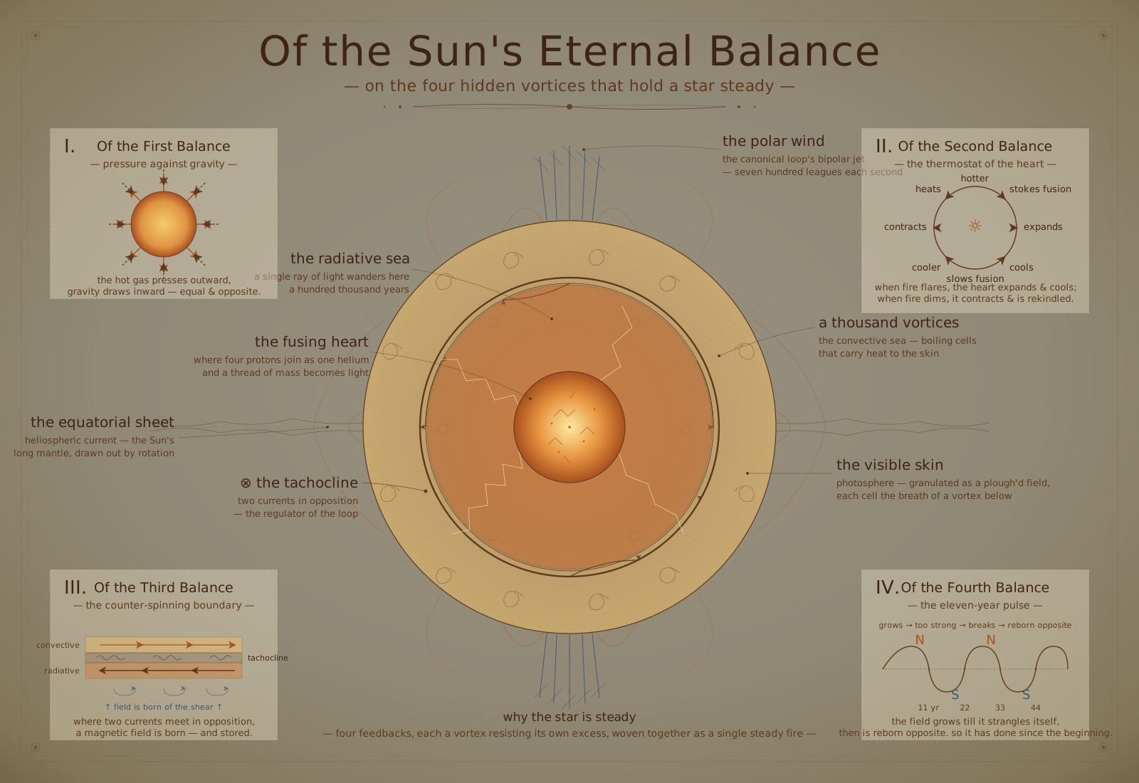
The Argument in Brief
The substrate’s energy organizes into a canonical topology at every scale: a co-rotating disk, polar jets, counter-rotating boundary layer, radiated waves. This chapter argues that the Sun’s observed structure, dynamics, and energy output are the canonical loop expressed in stellar plasma, with the substrate providing the organizational scaffolding that standard magnetohydrodynamics (MHD) describes but does not explain.
The Sun has differential rotation (the equator laps the poles by ~30%), an 11-year magnetic polarity cycle, polar coronal holes with fast wind streams, an equatorial current sheet, explosive flares and coronal mass ejections, and a convective interior that somehow maintains coherent large-scale magnetic fields against turbulent diffusion. Each of these features maps onto a component of the canonical loop. The substrate framework does not replace standard solar physics — the MHD equations, the nuclear reaction networks, the convective zone models are all correct descriptions of what the plasma does. What the framework adds is a structural argument for why the plasma organizes itself this way, and a set of quantitative connections that link solar observables to substrate parameters already fixed by particle physics and cosmology.
The Sun as Canonical Loop
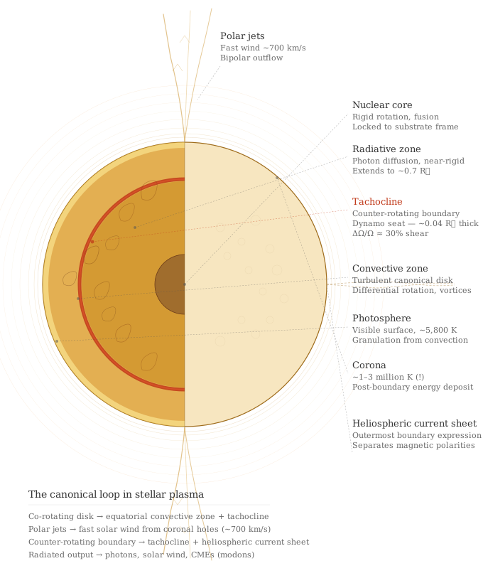
Standard solar structure
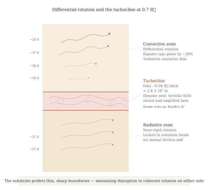
The Sun’s interior divides into three zones: a radiative core (center to ~0.7 R_\odot), where energy transport is dominated by photon diffusion; a convective envelope (~0.7 R_\odot to the surface), where energy transport is dominated by turbulent convection; and the tachocline at ~0.7 R_\odot, a thin shear layer where the radiative zone’s rigid-body rotation transitions to the convective zone’s latitude-dependent differential rotation.
Above the surface: the photosphere (visible surface, ~5,800 K), the chromosphere (~10,000 K), the transition region (rapid temperature jump), and the corona (~1–3 million K). The corona’s anomalously high temperature — hundreds of times hotter than the surface — remains one of the outstanding puzzles of solar physics.
The canonical loop mapping
| Component | Solar structure | Canonical loop |
|---|---|---|
| Co-rotating disk | Equatorial convective zone + tachocline | Accretion disk |
| Polar jets | Fast solar wind from coronal holes, ~750 km/s | Bipolar outflow |
| Counter-rotating boundary | Tachocline shear layer + heliospheric current sheet | Boundary sheath |
| Radiated output | Photons (luminosity), solar wind particles, CMEs | Modons / radiated waves |
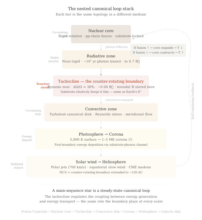
The mapping is not metaphorical. The tachocline is a physical shear layer — angular velocity changes by ~30% across a region only ~0.04 R_\odot thick. In the substrate framework, this is the counter-rotating boundary between the core’s rigid rotation (locked to the substrate’s deep frame-dragging) and the convective envelope’s differential rotation (driven by convective angular momentum transport). The tachocline is where the Sun’s large-scale magnetic field is generated and stored — it is the dynamo’s seat, the same role the counter-rotating boundary plays in the canonical loop at every other scale.
The Sun’s tachocline plays the same structural role as Earth’s D″ layer — both are counter-rotating boundaries between a rigidly rotating inner region and a differentially rotating outer region. Both are where the large-scale magnetic field is generated. The substrate framework predicts this correspondence: the canonical loop’s boundary sheath, expressed in whatever material is available (liquid iron for Earth, ionized plasma for the Sun), always becomes the dynamo seat.
Differential Rotation
What we observe
Helioseismology reveals the Sun’s internal rotation profile with remarkable precision. The equator rotates with a period of ~25 days; the poles with a period of ~35 days. This differential rotation persists throughout the convective zone (~0.7–1.0 R_\odot) but vanishes sharply at the tachocline — below it, the radiative zone rotates nearly rigidly.
The rotation profile is approximately:
\Omega(\theta) \approx \Omega_\text{eq}\,(1 - \alpha_2\cos^2\theta - \alpha_4\cos^4\theta)
where \theta is co-latitude, \Omega_\text{eq}/(2\pi) \approx 460 nHz (~25.4-day period), \alpha_2 \approx 0.14, and \alpha_4 \approx 0.15. The equator-to-pole angular velocity contrast is \Delta\Omega/\Omega_\text{eq} \approx 0.29.
What standard physics says
Standard solar physics explains differential rotation through the interaction of convection, rotation, and the meridional circulation. The Reynolds stresses from turbulent convection transport angular momentum equatorward, spinning up the equator. Mean-field hydrodynamic models (the \Lambda-effect) reproduce the surface differential rotation reasonably well, though the details of the tachocline’s maintenance remain debated.
What the substrate adds
The substrate framework adds a structural observation: the equatorial speedup is the expected geometry of a co-rotating disk in an elastic medium. In the feedback topology, the canonical loop organizes angular momentum into a planar structure — the co-rotating disk — where equatorial flows are faster because the medium’s sheet geometry (the local chirality-coherent plane) preferentially supports in-plane motion.
The quantitative question is whether the substrate’s sheet stiffness contributes measurably to the observed differential rotation, or whether it is entirely accounted for by the convective Reynolds stresses. The substrate’s contribution would appear as a latitude-dependent restoring force on angular momentum perturbations — an elastic term in addition to the turbulent viscous term. This is a small correction to a large effect, and detecting it would require extremely precise helioseismic inversions.
The more striking substrate contribution is to the tachocline’s thinness. Standard MHD predicts that the tachocline should spread inward through magnetic diffusion on a timescale much shorter than the Sun’s age. The fact that it remains thin (~0.04 R_\odot) requires a confinement mechanism. The leading standard explanation is a weak internal magnetic field that resists spreading. The substrate framework offers an alternative or complementary mechanism: the tachocline is a counter-rotating boundary whose thickness is set by the balance between the boundary’s internal shear energy and the substrate’s elastic restoring force. The substrate prefers thin, sharp boundaries because they minimize the disruption to the lattice’s coherent rotation on either side.
The tachocline confinement argument is qualitative. Computing the substrate’s contribution to tachocline thickness requires solving the HVBK equations for a counter-rotating boundary embedded in a stellar plasma — a calculation that has not been performed. The standard magnetic confinement mechanism (Gough & McIntyre 1998) may be sufficient. The substrate framework predicts that both mechanisms contribute, with the substrate’s contribution dominant at scales below the local \xi.
The Solar Magnetic Cycle
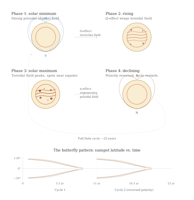
The 22-year Hale cycle
The Sun’s magnetic field reverses polarity approximately every 11 years, with a full magnetic cycle (return to original polarity) of ~22 years. The cycle manifests as the butterfly diagram — sunspots appear at mid-latitudes early in the cycle and migrate toward the equator as the cycle progresses. At solar maximum, the poloidal (dipolar) field weakens and reverses; the toroidal (sunspot-producing) field peaks.
Standard dynamo theory explains this through the \alpha–\Omega mechanism: differential rotation (\Omega-effect) stretches the poloidal field into a toroidal field; helical convective motions (\alpha-effect) regenerate the poloidal field from the toroidal. The tachocline stores and amplifies the toroidal field. The equatorward migration of sunspots reflects the equatorward propagation of a dynamo wave.
Substrate interpretation of the cycle
In the substrate framework, the solar magnetic cycle is a boundary layer oscillation — the counter-rotating boundary (tachocline) oscillates between two states of opposite polarity, with the oscillation driven by the same feedback mechanism that produces oscillations in boundary layers at other scales.
This is the anti-phase breath at stellar scale. The lattice’s like objects lock into an anti-phase oscillation — the Cooper pair and the lattice’s own breath, each vortex shadowed by a counter-rotating partner that exchanges energy across a shared seam rather than dissipating it. The tachocline does the same thing one tier up: it breathes between opposite-polarity states, the toroidal field handing its energy to the poloidal and back, which is why the cycle is a lossless self-sustaining oscillation rather than a damped one. By the substrate ladder’s sign rule this is the locking pole at stellar scale — a structure whose job is to bind and exchange energy sits on a tooth — and the toroidal-to-poloidal handoff is the ladder’s lossless coin circulating on a 22-year clock. The Sun’s faster breath is acoustic — the five-minute p-mode oscillations helioseismology reads, the whole star ringing in and out — while the 22-year polarity cycle is the slow anti-phase breath at the tachocline’s far longer diffusion clock. Those p-modes are a ladder of a different kind from the substrate’s own: the Sun is a bounded acoustic cavity with a definite size, so it rings in a harmonic comb — overtones spaced evenly in frequency by the large separation \Delta\nu — the length-bearing complement to the substrate’s lengthless \sqrt2 tower, the same keyboard-versus-string distinction the ladder draws for coronal loops and crystal lattices: a system with a length makes overtones, while the substrate, with no length of its own between its cutoffs, makes only the \sqrt2 ratio.
The key insight is from the galactic dynamics chapter’s current-phase relation (CPR). The counter-rotating boundary has a parity-symmetric CPR — it does not intrinsically prefer one magnetic polarity over the other. The system oscillates between them because the dynamo feedback is self-limiting: the toroidal field grows until it becomes strong enough to backreact on the differential rotation (quenching), at which point the \Omega-effect weakens, the toroidal field decays, and the poloidal field (regenerated by the \alpha-effect) sets the stage for the opposite polarity. This is precisely the behavior of a driven oscillator in a parity-symmetric potential — the system cannot settle into either polarity and instead oscillates between them.
The substrate’s contribution is to explain why the oscillation period is ~22 years and why it is so regular (the cycle length varies by only ~20% over centuries of observation). The oscillation timescale is set by the magnetic diffusion time across the tachocline, which in turn depends on the boundary layer’s thickness and conductivity. The substrate’s elastic restoring force on the boundary layer acts as a stabilizing influence, reducing the sensitivity of the period to turbulent fluctuations in the convective zone — the same stabilization mechanism that the Gaia chapter invokes for Earth’s geodynamo.
The magnetic diffusion time across the tachocline: \tau_\text{diff} = \frac{d_\text{tach}^2}{\eta_\text{eff}} with d_\text{tach} \approx 0.04\,R_\odot \approx 2.8 \times 10^7 m. Used with the bulk convective-zone turbulent diffusivity \eta_\text{turb} \approx 10^{8}–10^{9} m²/s, this gives only \tau_\text{diff} \sim 0.02–0.2 years — far shorter than the cycle, which is the familiar reason a decadal clock cannot be the bulk turbulent diffusion time. Reproducing the observed $$11-year half-cycle requires the effective diffusivity at the boundary to be suppressed by \sim 30–100\times to \eta_\text{eff} \sim 10^{6}–10^{7} m²/s, which gives \tau_\text{diff} \sim 1–8 years. That suppression is exactly what the substrate’s elastic stiffening of the counter-rotating boundary supplies: a stiffer boundary carries a lower effective diffusivity, lengthening the period from the too-fast bulk value toward the observed decade.
Solar Flares and CMEs: Boundary Layer Disruptions
What we observe
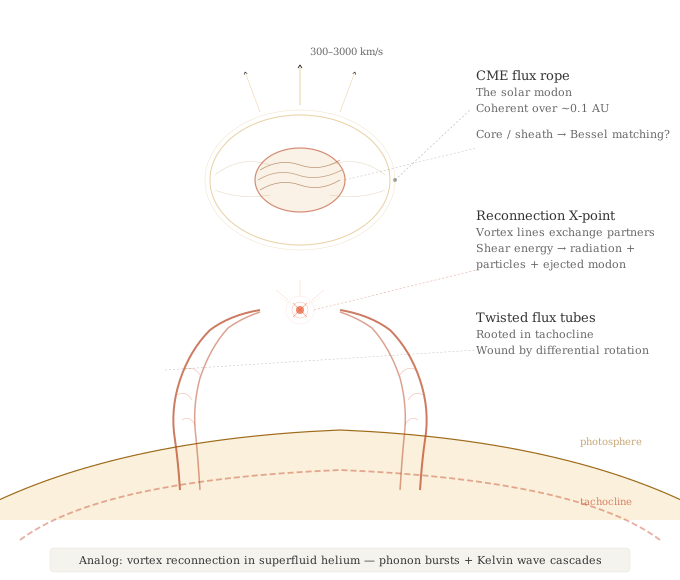
Solar flares are explosive releases of energy (10^{20}–10^{25} J per event) in the corona, associated with magnetic reconnection in twisted flux tubes. Coronal mass ejections (CMEs) are billion-ton blobs of magnetized plasma ejected into the heliosphere at speeds of 300–3000 km/s. Both are concentrated near the solar equator during solar maximum, when the toroidal magnetic field is strongest.
Substrate interpretation
In the substrate framework, flares and CMEs are boundary layer disruptions — localized failures of the counter-rotating boundary’s coherence, where stored magnetic (rotational) energy is suddenly released as propagating disturbances.
The analogy is to vortex reconnection events in superfluid helium. When two counter-rotating vortex lines approach closely enough, their cores can reconnect — exchanging partners and releasing the stored shear energy as phonon bursts and Kelvin wave cascades along the reconnected filaments. The physics is well-studied experimentally (Bewley, Paoletti et al. 2008) and computationally (Villois, Proment & Krstulovic 2017).
In the Sun, the “vortex lines” are magnetic flux tubes rooted in the tachocline, twisted by differential rotation and convective buffeting until they become unstable. Reconnection releases the stored shear energy as: (1) radiation across the spectrum (the flare), (2) accelerated particles (the energetic particle event), and (3) ejected plasma blobs (the CME).
The CME is the solar analog of the modon. A CME is a coherent magnetic structure — typically a flux rope — that propagates outward through the solar wind, maintaining its internal coherence over scales of ~0.1 AU. In substrate terms, it is a large-scale vortex dipole ejected from the boundary layer, carrying excess angular momentum and magnetic energy downstream — exactly the function of the modon in the canonical loop.
The substrate framework predicts CMEs are modon-like: a J_1-Bessel interior matched to a decaying K_1 exterior at a characteristic boundary. The interior side of this prediction is independently corroborated by standard solar physics. Magnetic clouds (the flux-rope core of a CME) are routinely fit by the Lundquist (1950) force-free solution [R80] B_z(r) = B_0\,J_0(\alpha r), \qquad B_\phi(r) = B_0\,J_1(\alpha r), \qquad B_r = 0 — exactly the J_0/J_1 Bessel pair that defines the modon interior in the framework. Lepping, Jones & Burlaga (1990) [R81] introduced the constant-\alpha force-free fit to 1-AU magnetic-cloud passes (typical cloud diameter 0.2–0.4 AU, peak field 15–30 nT) and reported good agreement on the smooth field rotation through the cloud; subsequent Wind / ACE / STEREO catalogs (reviewed in Kilpua, Koskinen & Pulkkinen 2017 [R82]) have applied the same fit to several hundred events. The framework reads this as evidence that magnetic clouds are bona fide Bessel ropes — the same structural family as the photon modon, scaled up by ~10^{17} in radius.
The literal interior/exterior radius ratio, by contrast, does not match the modon picture. Statistical surveys give a mean upstream sheath thickness of ~0.13 AU vs a mean MC radial width of ~0.29 AU [R82], implying a sheath/MC width ratio of ~0.45 (equivalently, total-extent / core-radius ~1.9), with factor 2–3 event-to-event scatter and no characteristic value near j_{11} \approx 3.83 [R82, R83]. A CME’s upstream sheath is shock-compressed ambient solar wind, dynamically assembled as the flux rope plows through the heliosphere — not the modon’s freely decaying K_1 tail. The two structures share a name (interior + sheath) but not a mechanism, and folding them into a single Bessel-matching prediction was the wrong move. The framework’s testable content is the interior force-free Bessel structure (which the data support), not the outer ratio.
Coronal heating
The corona’s anomalous temperature (\sim 10^6 K vs the photosphere’s \sim 5800 K) has resisted explanation for decades. The two leading candidates are wave heating (MHD waves from the convective zone dissipating in the corona) and nanoflare heating (a myriad of tiny reconnection events releasing energy continuously).
The substrate framework does not add a third heating channel. An HVBK mutual-friction estimate of energy deposition from the dc1 lattice into the coronal plasma, \dot q \sim \alpha_{mf}\,\rho_{DM}\,\omega_0\,|\Delta v|^2, gives \dot q \sim 10^{-12} W/m³ for plausible substrate-plasma slip velocities (|\Delta v|\!\sim\!10^3 m/s) — roughly six orders of magnitude below the \sim 3\times 10^{-6} W/m³ required to produce the empirical quiet-Sun budget of \sim 300 W/m² over a 10^8 m scale height. Reaching the budget would demand |\Delta v|\!\to\!v_L, which is the saturation condition used in the fast wind argument, not an independent steady-state heating mechanism. The standard wave + nanoflare picture is sufficient.
What the framework does contribute is a structural reason why those mechanisms operate so effectively here. The corona is the region outside the Sun’s primary counter-rotating boundary (the tachocline and its magnetic extension into the atmosphere), and in the canonical loop the post-boundary region is where expelled energy — modons, radiated waves, excess angular momentum — deposits into the surrounding medium. The coronal temperature reflects that continuous deposition; the standard wave and nanoflare channels are how it shows up in the plasma.
The Solar Wind and the Heliosphere
The canonical loop’s radiated output
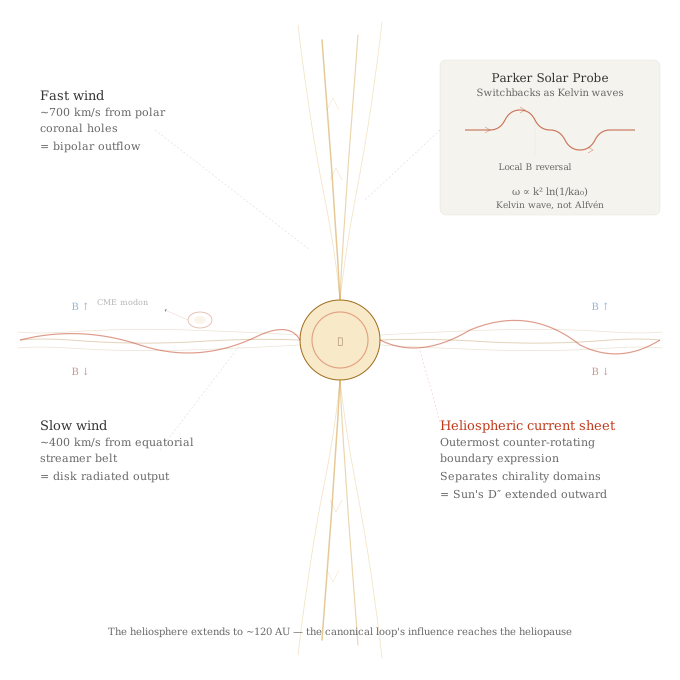
The solar wind is the Sun’s radiated output — plasma expelled continuously from the corona at 300–800 km/s, carrying magnetic field, angular momentum, and energy into the heliosphere. The wind has two distinct components:
Fast wind (~750 km/s): emerges from polar coronal holes — regions of open magnetic field lines over the Sun’s poles. In the canonical loop, these are the polar jets. The fast wind is relatively steady, low-density, and carries a magnetic field aligned with the Sun’s dipole axis. Its speed is no accident in the framework: it is the same substrate critical velocity v_L = \omega_0\xi that sorts galaxies from clusters, measured here in our own back yard (Ulysses high-latitude mean 751.5 km/s) — see Galactic Dynamics § What Sets the Critical Velocity for why one number ties these disconnected domains together.
Slow wind (~400 km/s): emerges from near the equatorial streamer belt and the boundaries of coronal holes. It is denser, more variable, and magnetically disordered. In the canonical loop, the slow wind is the disk’s radiated output — material shed from the co-rotating equatorial structure and its boundary regions.
That the fast polar jet launches at the outer critical rim v_L = 0.0025\,c — rather than the inner relativistic rim a black hole’s jet reaches — has a sharp consequence in the substrate’s information architecture: read as a four-port node, the Sun’s coherent catchable leak (its modon coin, the CME) is suppressed by the launch compactness to \kappa/g = \beta_c^5 \approx 10^{-13} of the drive. The Sun is thus the canonical producer’s outer-rim endpoint — a bare thermal radiator whose non-drive output is overwhelmingly incoherent photon luminosity — the opposite end of the same law from an AGN, which launches relativistically and leaks \sim 10\% of its source as a coherent coin. Same loop, opposite rim; the rim sets the leak.
Fast wind terminal velocity = v_L
The fast wind’s terminal velocity is the cleanest cross-scale numerical match the substrate framework makes in stellar physics. The Ulysses SWOOPS instrument, in three polar passages over a full solar cycle, measured the average fast wind speed at high latitude (70°–90°) from polar coronal holes:
| Solar minimum | Mean high-latitude fast wind speed | Reference |
|---|---|---|
| Cycle 22 (Ulysses 1st orbit, 1994–95) | \mathbf{763} km/s | McComas et al. 2000 [R76] |
| Cycle 23 (Ulysses 3rd orbit, 2007–08) | \mathbf{740} km/s | McComas et al. 2008 [R77]; Ebert et al. 2009 [R78] |
| Single deep-coronal-hole rotation | 780 \pm 17 km/s | Goldstein et al. 1996 |
| Mean of cycles 22 and 23 | \mathbf{751.5} km/s | — |
The substrate prediction, from the same parameters that fix the CDM-to-MOND transition at galactic scale:
v_L = v_\text{rot,outer} = \omega_0\xi = 0.0025\,c = \mathbf{749.5}\;\text{km/s}
Match: 0.3% on the cycle-averaged mean; ~2% on individual cycles. This is comparable precision to the bridge equation’s MOND match (~3% on a_0), and the same v_L appears on both sides of the comparison — set by substrate parameters (\omega_0, \xi) fixed independently by electroweak physics and condensate microphysics (galactic dynamics).
In the canonical loop picture, this is not a coincidence: the polar jet is the loop’s mechanism for exhausting excess angular momentum, and the substrate cannot sustain organized flow above v_L before quasiparticle excitation begins to dissipate it. Once the wind accelerates to v_L, further acceleration costs energy to the substrate’s vortex modes faster than the coronal-hole driver can supply it; the wind saturates.
Read through the ladder’s coin, this is the same Landau ceiling the lightning chapter meets one regime down. Below v_L the organized flow rides the substrate’s lossless channel — the paired anti-phase breath — and pays nothing to move; at v_L that breath can no longer complete its handoff inside the light cone, the exchange goes lossy, and the excess is spent to vortex modes. Lightning spends it as a shed gamma modon when an electron crosses 0.776\,c; the polar jet spends it as a velocity ceiling at 0.0025\,c — one mechanism, two scales.
Wave-turbulence-driven models (Cranmer 2002; Cranmer et al. 2016) reproduce the observed fast wind speed by tuning the Alfvén wave amplitude and reflection coefficient at the photospheric base. The terminal speed in those models is a fitted quantity — it is the speed that emerges from a particular choice of boundary conditions, not a first-principles prediction. The substrate framework predicts the same number from \omega_0 and \xi, parameters that are not tuned to fit solar wind observations. The two pictures are not in tension: standard MHD describes how the wind accelerates (Alfvén waves doing work against gravity); the substrate predicts where it has to stop.
The 3% drop in fast wind speed between cycles 22 and 23 minima (763 → 740 km/s) is small but real [R77, R78]. If the wind speed is rigorously set by v_L, this variation must reflect either (i) a real cycle-scale variation in \omega_0 or \xi — which the framework treats as constants — or (ii) the wind not quite reaching saturation in the weaker cycle. Option (ii) is the natural reading: the substrate sets a ceiling, and a weaker driver (the cycle-23 minimum was the deepest in 50 years) produces a wind that approaches but does not fully reach v_L. The framework predicts that high-latitude fast wind speed at the next deep solar minimum should be bounded above by v_L \approx 750 km/s and approach it more closely when the polar coronal hole driver is stronger. A measurement of fast wind speed exceeding v_L at high latitude in a normal coronal hole would falsify this aspect of the framework.
The heliospheric current sheet
The two wind components are separated by the heliospheric current sheet (HCS) — a thin, warped surface extending from the Sun’s magnetic equator throughout the heliosphere. The HCS is the Parker spiral’s organizing structure: above it, the magnetic field points one way; below it, the other. During solar minimum, the HCS is nearly flat and close to the ecliptic; during solar maximum, it becomes highly warped, following the Sun’s tilted and complex magnetic equator.
In substrate terms, the HCS is the outermost expression of the Sun’s counter-rotating boundary. It separates two domains of opposite magnetic polarity — two regions of the dc1 lattice with opposite chirality alignment. The HCS is to the Sun what the D″ layer is to Earth: the counter-rotating boundary extended outward into the surrounding medium.
Parker Solar Probe observations: switchbacks
The Parker Solar Probe (launched 2018) has measured the solar wind closer to the Sun than any previous mission, reaching below 15 R_\odot. Among its discoveries: switchbacks — rapid, Alfvénic reversals of the magnetic field direction that pervade the young solar wind (Bale et al. 2019 [R89]; Kasper et al. 2019 [R90]). These are localized S-shaped kinks in the magnetic field, propagating outward, with \delta v and \delta\mathbf{B}/\sqrt{\mu_0\rho} correlated in the sign expected for outgoing Alfvénic perturbations.
Recent statistics put concrete numbers on the population. From PSP encounters 1 and 2 inside 0.25 AU, Larosa et al. (2021) [R91] find a mean switchback width of \sim 5 \times 10^4 km, a mean length-to-width aspect ratio of \sim 28 (range 11–59), and a duration distribution that is a power law with tail slope \approx -2 from seconds to hours. Liu et al. (2023) [R92] track the radial evolution and find that switchback transverse size scales as R while radial size scales as R^2 — aspect ratios sharpen with heliocentric distance. About 27% of catalogued switchbacks are compressible (non-purely-Alfvénic) (Larosa et al. 2021 [R91]).
In the substrate framework, switchbacks are substrate-scale perturbations — Kelvin wave excitations on the magnetic vortex filaments extending from the Sun. When a vortex filament in a superfluid is perturbed, the perturbation propagates as a helical wave along the filament, with the local vortex line temporarily reversing its axial direction at the wave crest. The magnetic field reversal in a switchback is the plasma-scale manifestation of this substrate-scale vortex wave.
The leading standard interpretation is that switchbacks are spherically polarized large-amplitude Alfvén waves (Mallet et al. 2021 [R93]; Squire et al. 2022 [R94]) — coherent magnetic perturbations of constant |\mathbf{B}| that propagate along the background field at the local Alfvén speed v_A. This ansatz is non-dispersive by construction: every wavelength rides at v_A, and the observed Alfvénicity (\delta v \approx \pm \delta b/\sqrt{\mu_0\rho}) is automatic.
What discriminates the two pictures
The key observation is that the existing “Alfvénic” identification is not a direct dispersion measurement. It is inferred from \delta v/\delta b amplitude correlation, which any transverse fluctuation of an outgoing wave packet satisfies in the small-amplitude limit, including a Kelvin wave on a magnetic-vortex filament. I have not found a published study that plots \omega(k) for switchbacks directly** — the dispersion \omega = k v_A is assumed when applying Taylor’s hypothesis (Bourouaine & Perez 2020 [R95]; Perez et al. 2021), not measured.
The clean discriminator is wavelength-dependent phase speed:
- Alfvén (standard): \omega = k v_A, so v_\phi is independent of k. All switchback widths advect at the same speed in the plasma frame.
- Kelvin (substrate): \omega = (\Gamma k^2 / 4\pi)\left[\ln(2/ka) + \mathcal{O}(1)\right], so v_\phi = (\Gamma k/4\pi)\ln(2/ka). Shorter switchbacks travel faster than longer ones; the scaling is approximately v_\phi \propto 1/\lambda with a logarithmic correction.
For the relevant PSP regime — switchback wavelengths \lambda \sim 10^4–10^5 km and a plausible underlying filament core radius a \sim 10^3 km (set by photospheric flux-tube and granular scales; Fargette et al. 2021 [R96] traced switchback patches back to both granular \sim 10^3 km and supergranular \sim 3\times 10^4 km footpoint structure) — the dimensionless parameter ka runs \sim 0.06–0.6, well inside the Local Induction Approximation’s validity range, with \ln(2/ka) \approx 1–3.5 (an order-unity factor, not a free parameter once a is fixed).
Observable. Bin catalogued switchbacks at a fixed encounter by radial width \lambda (or duration \tau \approx \lambda/v_{sw}) and plot the plasma-frame propagation speed v_\phi^{(\text{pf})} = |v_\text{sw}^{(\text{sc})} - v_\text{sw}^{(\text{bg})}| - v_A inside each bin against \lambda.
Alfvén prediction: flat — slope 0 in \log v_\phi vs \log\lambda.
Kelvin prediction: slope \approx -1 (with mild logarithmic curvature). A switchback at \lambda = 5\times 10^3 km should propagate \sim 8–10\times faster in the plasma frame than one at \lambda = 5\times 10^4 km, after the logarithmic factor \ln(2/ka) is taken out.
Falsifier. A scatter plot showing no statistically significant width-vs-speed slope in a sample of \gtrsim 10^3 catalogued switchbacks at a single encounter falsifies this aspect of the framework. The Larosa et al. (2021) [R91] catalog already has enough events to do this; the analysis to my knowledge has not been published.
Cross-radial test. Because Kelvin-wave dispersion depends on substrate parameters (\Gamma, a) and not on v_A, the slope of v_\phi vs \lambda should be the same across PSP encounters at different heliocentric distances, even though v_A varies by factors of several between 0.05 AU and 0.3 AU. The Alfvén picture predicts that the intercept tracks v_A(R) while the slope stays zero. Liu et al. (2023) [R92] already report systematic radial evolution of switchback geometry but did not test the dispersion.
The dominant interpretation in the PSP literature (Mallet 2021 [R93]; Squire 2022 [R94]; recent reviews) is that switchbacks are spherically polarized Alfvén waves, a model whose non-dispersiveness is an assumption, not an empirical finding. Existing \delta v / \delta b Alfvénicity tests do not discriminate that model from a Kelvin-wave filament model, because both satisfy the same amplitude relation at the linear level. The substrate framework’s specific prediction — width-dependent plasma-frame phase speed — has not been tested. Boundary-layer surface waves at switchback edges are sometimes treated as Kelvin–Helmholtz unstable shear layers (Krasnoselskikh et al. 2020; Sioulas et al. 2025), but no published work to my knowledge has tested \omega \propto k^2\ln(1/ka) for the switchback body itself. Until that test is performed, the prediction in this chapter is best read as unfalsified, not confirmed.
Fusion in the Substrate Framework
Standard nuclear fusion
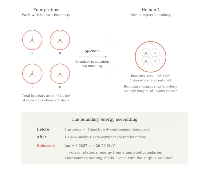
The Sun’s energy source is the proton-proton (pp) chain: four protons fuse into one helium-4 nucleus, releasing 26.73 MeV per reaction (mostly as kinetic energy of the products and neutrinos). The rate is governed by quantum tunneling through the Coulomb barrier and the weak interaction (p + p \to d + e^+ + \nu_e), which converts a proton to a neutron. The core temperature (~15.7 million K) provides the thermal energy for tunneling, and the rate is exquisitely sensitive to temperature: \epsilon \propto T^4 for the pp chain.
The substrate framework does not modify the nuclear reaction rates or the quantum tunneling probabilities. The pp chain is computed from the Standard Model’s electroweak and strong interactions, which the substrate framework reproduces in its own language but does not alter in their numerical predictions.
What the substrate adds: the tunneling environment
Where the substrate framework contributes is in the environment in which tunneling occurs. In the proton core chapter, the proton is a three-fold Y-junction of interlocking quark orbital systems, enclosed by a confinement boundary (Layer 2) that stores ~929 MeV of counter-rotating boundary energy. When two protons approach each other, their confinement boundaries interact.
In standard QFT, the Coulomb barrier is an electrostatic potential energy hill: V(r) = e^2/(4\pi\epsilon_0 r). The protons tunnel through this barrier via quantum mechanical amplitude. In the substrate framework, the Coulomb barrier is a boundary interaction — the outermost counter-rotating layers of the two protons’ orbital systems encountering each other, with the repulsive force arising from the difficulty of merging two counter-rotating boundaries of the same polarity.
The tunneling event is then a boundary layer penetration: the dc1 condensate at the boundary between the two protons momentarily thins enough — through the stochastic fluctuations of the counter-rotating eddies — for the two co-rotating cores to merge their flow fields. This is the same tunneling mechanism described in two-fluids quantum potential, now applied at nuclear scale where the boundary energies are \sim 10^5 times greater.
From protons to deuterium: the weak interaction as chirality flip
The first step of the pp chain requires one proton to become a neutron: p \to n + e^+ + \nu_e. In the Standard Model, this is a weak interaction — a W^+ boson mediates the transformation. In the substrate framework, the weak interaction is a chirality flip in the dc1 substrate’s local ordering (see Higgs field). The up quark (+2/3, Type A orientation at the Y-junction) transforms into a down quark (-1/3, Type B orientation) — a reorientation of one branch of the proton’s three-fold junction from axis-aligned to axis-perpendicular.
This reorientation is suppressed because it requires rotating a quark’s orbital plane through the junction’s confining potential — a process whose rate is governed by the local Higgs field (chirality ordering) and the weak coupling constant. The extreme slowness of this step (~10^{10} years for any given proton in the solar core to undergo it) is the rate-limiting factor for solar fusion, and the substrate framework inherits this timescale from the Standard Model without modification.
Helium-4 as a closed topology
The fusion product — helium-4 — has a notable property in the substrate framework. Its two protons and two neutrons form a closed topological system: two uud junctions and two udd junctions, interlocked with paired spins. The helium-4 nucleus is the tightest-packed baryon system — a doubly-magic nucleus with all angular momenta paired. In substrate terms, it is a boundary-minimizing configuration: the four baryons arrange their counter-rotating boundaries so as to minimize the total boundary surface area, which minimizes the total stored boundary energy.
The 26.73 MeV released per fusion event is, in the substrate picture, the excess boundary energy liberated when four separate protons (each with its own confinement boundary) merge into one helium-4 nucleus (with a single, more compact boundary). The mass deficit \Delta m = 0.0287\;u is the rotational energy that was stored in the now-eliminated boundary layers — four boundaries replaced by one, with the excess radiated as kinetic energy and modons. In the ladder’s economy this is where the Sun mints the coin: the boundary merger releases the lattice’s paired breath, which then propagates outward and is spent through the three channels of thermal dynamics — radiation, conduction, and convection — that carry the energy from core to photosphere.
Interactive: the chain, run — p + p seaming with the flip in the act (the positron shed), then He-3, then He-3 + He-3 closing into the alpha and freeing two protons, each rung’s excess boundary energy leaving as modons; the seam view shows why two bare protons are turned back.
Two structural facts about nuclear binding — which standard nuclear physics absorbs as empirical inputs — follow directly from the substrate’s boundary picture. The first is why nuclear binding is so small. The counter-rotating boundary that confines three quarks into one nucleon stores ~929 MeV (the proton core mass budget), yet a nucleon joining the helium-4 cluster gives up only ~7 MeV — a factor of ~130 less. This is expected: a free nucleon is already a closed, color-singlet boundary, so when two nucleons approach, only the tails of their counter-rotating boundaries overlap. Confinement is the full boundary — \sigma acting over a full femtometer of flux tube; nuclear binding is a residual, van-der-Waals-like overlap of two already-saturated boundaries. The ~100× suppression is what QCD calls “confinement versus the residual strong force,” read here as “full boundary versus boundary-tail overlap.”
The second fact is why binding saturates — why it tracks the number of nucleons (the volume term a_V \approx 16 MeV/nucleon of the semi-empirical mass formula) rather than the number of nucleon pairs. Saturation is the nuclear analog of the constant string tension. In the proton core chapter, \sigma is independent of flux-tube length because it is fixed by local substrate properties at the boundary, not by the global configuration. The same locality makes a boundary merger a contact interaction: each nucleon shares boundary only with its immediate neighbors, so an interior nucleon binds to a fixed number of partners no matter how large the nucleus grows. Constant energy per shared boundary gives constant binding per nucleon. Boundary locality is the single mechanism behind both — the constancy of \sigma inside a nucleon and the saturation of binding between nucleons.
An earlier version of this check estimated the binding from the reduction in outer surface area, E_\text{bind} \approx \sigma\,\Delta A with \Delta A \approx 2.6 fm², and reported ~2.3 MeV. That had two flaws. Dimensionally, \sigma \approx 0.9 GeV/fm is an energy per unit length (a tension), not per unit area — multiplying it by an area is not an energy. Physically, the four-proton and helium-4 boundary energies are each \sim GeV (~929 MeV/nucleon of confinement), and the binding is the \sim 0.75\% difference between them; a 0.75% difference cannot be recovered by subtracting two multi-GeV surface energies estimated to few-fm² precision. Binding must be computed as the boundary reorganization, not as a difference of bulk areas.
The dimensionally correct object is flux-tube length. The confinement budget gives each nucleon an energy-weighted internal flux-tube length L_Y \approx E_\text{conf}/\sigma, and binding is B = \sigma\,\Delta L. The energy to use here is the stored boundary energy, not the visible mass: the proton presents N\approx1836 seams each leaking \alpha_{mf}=0.3008, so it stores \approx 3.12 GeV and shows 938 MeV (Proton Core § The Universal Effective Quantum). That gives L_Y \approx 3110/900 \approx 3.46 fm, or \approx 1.15 fm per Y-junction arm. The observed B = 28.3 MeV then corresponds to \Delta L = B/\sigma \approx 0.031 fm across the whole four-nucleon cluster — a \sim 0.22\% shortening of its \approx 13.8 fm total boundary network. (That is the shortening relative to stored boundary energy; the familiar \sim 0.76\% figure is the mass defect B/M, a different ratio and unchanged.)
This equals B/E_\text{conf} identically, so it is a consistency check, not a prediction: computing \Delta L from the merged-cluster geometry (the minimal connected flux-tube network spanning all twelve quarks, versus four separate Y-strings) is Open Problem #2. The deuteron — one shared boundary — binds by 2.22 MeV, of order one effective quantum (m_\text{eff} = 1.70 MeV); but binding per shared boundary is not additive (helium-4’s six pair-bonds average 4.7 MeV, not 2.2), the cooperative excess being the closed-topology effect below, so per-bond counting is not yet predictive either.
What the framework does fix is the shape of the binding-energy curve. Mapping the semi-empirical mass formula onto substrate boundary energies — volume = saturated merger per nucleon (locality), surface = unmerged boundary on surface nucleons, Coulomb = same-polarity boundary repulsion, pairing = closed-topology bonus — the smooth liquid-drop value for helium-4 is ~22–25 MeV. Helium-4 falls below the bulk per-nucleon value (a_V \approx 16 vs. 7.07 MeV/nucleon observed) for a clean reason: it is all surface — all four nucleons are surface nucleons with unmerged boundary, so it never reaches the saturated bulk energy. The remaining ~3–6 MeV excess over the smooth value is the doubly-magic closed-topology bonus — the boundary-minimizing, all-spins-paired configuration named above, which the smooth formula misses and which the substrate picture requires precisely for the tightest-packed closed boundary.
What Makes the Sun’s Light
The Sun emits a near-perfect Planck curve, without spectral lines that is not typical for a gas that will have gaps or bands.
From the substrate’s perspective, Planck’s law needs three things: an indivisible modon with energy h\nu, a boundary geometry that circulates them so all are absorbed and re-emitted by a merged boundary. Once orbital boundaries have merged, they lose the spectral lines.
Spectral free radiation normally comes from condensed matter like graphite, soot, metal-black - the materials that absorbs light and emits it back as heat. Kirchhoff’s claim that any opaque enclosure at equilibrium contains black radiation is not correct [R204] — and Planck knew it in practice, because he had to drop a speck of carbon (a Kohlenstäubchen) into his perfectly reflecting cavity to make the radiation thermalize at all. He called the speck a catalyst - but it was really a perfect absorber.
These materials have merged orbital boundaries, like metals as described in the conductors section. Once the orbital boundaries have merged, they lose the specific gaps that create the spectral lines. Instead continuous boundaries create continuous spectra.
The Sun’s carbon speck is H^-
The Sun’s photosphere is not a metal and doesn’t fit exactly. What it does have though is the H^- ion layer. Hydrogen so weakly holds an extra electron that the orbital is already effectively a continuum. This makes every H^- ion a broadband absorber and emitter, the Sun’s equivalent of the speck of carbon. Although there is only one H^- ion per 10^8 hydrogen atoms, they are embedded in a layer thick enough that all emitted light is absorbed and reemitted many times over before a modon leaves.
The discriminator at 1.645 \mum
A condensed photosphere emits by directional spectral emissivity — the angular pattern a real material presents, set by its refractive index, which varies slowly and smoothly with wavelength. It has no reason to know about any particular photon energy.
An H^- photosphere emits through a seam with a threshold. Below 0.754 eV the second electron cannot be ejected, so the bound-free channel switches off abruptly at \lambda = 1.645\;\mum and only the weaker free-free channel remains. The total continuous opacity therefore has a sharp minimum near 1.6\;\mum — the \tau=1 surface moves downward into hotter gas, we see some tens of kilometres deeper into the Sun, and the limb darkening, which is a readout of the temperature gradient across the layer being sampled, is shallowest right there.
This is exactly what is observed, and it is why 1.6\;\mum is the band solar telescopes use to image the deepest visible photosphere. The Sun’s continuum limb darkening is strong in the blue, weakens through the red, reaches its minimum at the opacity minimum, and turns back up beyond it. A feature pinned at 1.645\;\mum, tracking a 0.754 eV binding energy, is a ladder signature — the fingerprint of a seam with a top. No lattice has a reason to produce one there.
If the framework’s reading is right, the wavelength of the solar opacity minimum is a measurement of the H^- electron affinity and must not move: it should sit at the same 1.6\;\mum in every star whose photosphere is inside the H^- window, independent of surface gravity, metallicity, or activity. A star with a solar-type photosphere whose opacity minimum sat somewhere else would break the identification.
Stellar Structure as Nested Canonical Loops
The core: rigid rotation locked to the substrate
The Sun’s radiative core rotates nearly rigidly — a striking observation given that the convective zone above it is differentially rotating. Standard explanations invoke the magnetic coupling between the core and the tachocline, or the angular momentum transport by internal gravity waves.
The substrate framework offers an additional mechanism: the core’s rotation is locked to the substrate’s local frame-dragging. The core’s angular momentum (J = I\Omega_\odot \sim 2 \times 10^{41} kg·m²/s for the radiative interior — note this is the angular momentum, not the moment of inertia I \approx 0.07\,M_\odot R_\odot^2 \approx 7 \times 10^{46} kg·m²) entrains the dc1 condensate through mutual friction, and the condensate’s response — a macroscopic rotation of the local substrate lattice — in turn provides a restoring torque that resists differential rotation. The result is rigid-body rotation at a rate set by the substrate’s steady-state mutual friction balance.
This is the same mechanism that the Gaia chapter invokes for Earth’s inner core, scaled up by \sim 10^{6} in mass and \sim 10^{2} in radius. The frame-dragging angular velocity at the Sun’s surface is:
\omega_\text{fd,\odot} = \frac{2GJ_\odot}{c^2 R_\odot^3} \sim 10^{-12}\;\text{rad/s}
This is many orders of magnitude below the Sun’s rotation rate (\Omega_\odot \sim 2.9 \times 10^{-6} rad/s), so the direct frame-dragging is negligible. The substrate’s coupling acts through the mutual friction channel — the same \alpha_{mf} parameter that governs boundary transmission at every other scale — which is far more efficient than gravitational frame-dragging alone.
The convective zone: a turbulent canonical disk
The convective zone is the Sun’s “accretion disk” — a turbulent, differentially rotating region where angular momentum is transported by Reynolds stresses and large-scale meridional flows. Giant convective cells (possibly the solar equivalent of Hadley and Ferrel cells in Earth’s atmosphere) organize the flow at large scales; granulation and supergranulation organize it at smaller scales.
In the substrate framework, the convective zone is a turbulent canonical disk whose structure is biased by the substrate’s sheet geometry. The substrate predicts that large-scale convective patterns should preferentially align with the substrate’s chirality-coherent planes — a subtle prediction that might manifest as a slight preference for convective cell alignment with the ecliptic plane.
A note on the Sun’s layers, read through the substrate ladder. The radial stack — core, radiative zone, tachocline, convective zone, atmosphere — is the canonical loop nested, but its scales are mechanism-set (by opacity, ionization state, and the dominant energy-transport mode), not by the substrate’s pairing ratio: it is the ladder’s coarse family, like the five scales of superconductivity or the temperature column of thermal dynamics, and not a \sqrt2 comb. The one place the Sun offers a candidate genuine ladder is the convective-cell hierarchy itself — granulation (\sim 1 Mm) \to mesogranulation \to supergranulation (\sim 30 Mm) \to giant cells — a discrete, log-spaced tower of turbulent scales. Whether those scales cluster, and on what ratio, is a comb test of the same kind the lightning branch-points offer: the clustering is the firm claim, the \sqrt2 ratio is open, and the family is coarse.
The corona and wind: post-boundary energy deposition
As discussed above, the corona is the post-boundary region where excess energy from the tachocline’s counter-rotating boundary is deposited. The solar wind is the canonical loop’s radiated output — modons and organized disturbances propagating through the heliosphere.
Stellar Formation in the Substrate
Gravitational collapse as substrate reorganization
Star formation begins with the gravitational collapse of a molecular cloud core. In the substrate framework, this is a reorganization of the dc1 lattice: the baryonic matter’s gravitational field (transmitted through the ebbing current mechanism of gravity) draws surrounding substrate into a denser configuration, compressing the lattice and increasing the local vortex density. The collapsing cloud’s angular momentum is organized by the substrate’s sheet geometry into the observed disk-jet morphology of protostellar systems.
The standard picture — cloud collapse, disk formation, bipolar outflow — is the canonical loop assembling itself from a diffuse initial state. The substrate’s contribution is to explain why every protostellar system exhibits this topology: the disk-jet-counterflow structure is the substrate’s preferred organizational mode for angular momentum at every scale, and gravitational collapse simply provides the energy to assemble it.
Jeans mass and the substrate
The Jeans mass — the minimum cloud mass for gravitational collapse — is
M_J = \rho \left(\frac{\pi c_s^2}{G\rho}\right)^{3/2}
where c_s is the thermal sound speed and \rho is the cloud density. The substrate does not modify this formula: the Jeans instability is a balance between thermal pressure and gravity, and the substrate’s elastic contribution to the effective pressure is negligible at molecular cloud densities (the substrate’s “stiffness” operates at the \xi scale, far below the Jeans length of \sim 0.1–1 pc).
However, the substrate does influence the fragmentation of collapsing clouds. The substrate’s sheet geometry provides preferred planes for filamentary fragmentation — and indeed, observations from Herschel and ALMA show that molecular clouds fragment into filaments, with characteristic widths of \sim 0.1 pc, before fragmenting further into individual cores. The substrate framework predicts that these filaments should preferentially align with the local substrate sheet structure, which in turn is aligned with the galactic disk’s midplane. This is consistent with observations showing that molecular cloud filaments are often aligned with the galactic plane, though the standard explanation (magnetic field alignment) is also viable.
The claim that substrate sheet geometry influences molecular cloud filament orientation competes with the well-established role of the galactic magnetic field. Disentangling the two requires regions where the magnetic field and the proposed substrate sheet orientation differ — a situation that may be rare if the magnetic field itself is organized by the substrate (as the galactic dynamics chapter suggests). This prediction may not be independently testable.
The Main Sequence and Stellar Evolution
Why stars are stable
A main-sequence star is a stable configuration: nuclear fusion in the core generates energy that balances gravitational contraction, with convective and radiative transport carrying the energy to the surface. The star sits in thermal and hydrostatic equilibrium.
In substrate terms, a main-sequence star is a steady-state canonical loop — the co-rotating core generates energy (fusion), the boundary layer (tachocline) regulates the coupling between core and envelope, and the radiated output (photons, neutrinos, wind) carries away the excess. The loop is self-regulating: if fusion increases, the core expands and cools, reducing the fusion rate; if fusion decreases, the core contracts and heats, increasing the rate. This thermostat is standard stellar physics, and the substrate framework does not modify it.
What the substrate adds is the observation that the thermostat’s feedback loop is an instance of the canonical loop’s self-regulation. The counter-rotating boundary (tachocline) acts as a regulator at the interface between energy generation and energy transport — the same role it plays in all canonical loops. The framework predicts that the tachocline properties (thickness, shear, magnetic field storage capacity) should correlate with the star’s position on the main sequence, with more massive stars having more energetic tachoclines (greater shear, stronger stored fields) because the larger luminosity requires a more vigorous canonical loop.
Stellar death and the boundary cascade
When a star exhausts its nuclear fuel, the canonical loop breaks down. The details depend on mass:
Low-mass stars (M \lesssim 8\,M_\odot): The core contracts to a white dwarf — a degenerate object supported by electron degeneracy pressure. The envelope is expelled as a planetary nebula. In substrate terms, the canonical loop’s energy source (fusion) shuts off, and the boundary cascade collapses: the tachocline disappears, the convective zone is expelled, and the remaining core settles into a minimum-energy configuration. A white dwarf is a frozen boundary — a compact object whose internal counter-rotating structure has been quenched by the loss of driving energy, leaving a degenerate state with no active canonical loop.
High-mass stars (M \gtrsim 8\,M_\odot): The core collapses beyond electron degeneracy to a neutron star or black hole, with the envelope expelled in a supernova. In the substrate framework, a core-collapse supernova is the most violent boundary disruption in the stellar catalog — the entire nested canonical loop structure of the star collapses in seconds, releasing \sim 3 \times 10^{46} J (mostly as neutrinos). The collapsing core’s counter-rotating boundaries are compressed to nuclear density, where the proton core’s three-fold junction topology (proton core) becomes the organizing structure. A neutron star is a macroscopic object organized at nuclear-scale boundary energies — the deepest tier of the substrate hierarchy promoted to stellar scale.
Neutron stars are the most interesting stellar objects from the substrate framework’s perspective. Their interior — a superfluid of neutrons and protons at nuclear density — is the closest macroscopic analog to the dc1 substrate itself. Pulsar glitches (sudden spin-up events) are attributed to vortex unpinning in the neutron superfluid interior — the same vortex dynamics that the substrate framework uses at every other scale. The framework predicts that pulsar glitch statistics (size distribution, waiting times) should follow the same scaling laws as vortex reconnection events in superfluid helium, modulated by the mutual friction parameter of the neutron superfluid. Note that the parameter entering here is a genuine per-boundary coupling and so obeys the Kopnin ceiling \alpha_{mf}\le\tfrac12 — the figure 552 used in earlier versions of this passage is the proton’s seam-count product N\alpha_{mf} (Mass as Leaking Rotational Kinetic Energy) and is not a dimensionless friction coefficient. Glitch phenomenology should be compared against the neutron-star mutual friction values of the pulsar literature, not against the count.
Predictions Specific to This Chapter
The following predictions extend the framework into solar and stellar physics. They are ordered from most to least testable with current or near-future data.
Fast solar wind terminal velocity bounded by v_L. The high-latitude fast wind from polar coronal holes should be bounded above by v_L = 0.0025\,c \approx 749.5 km/s and approach it when the polar driver is strong. Already observed in Ulysses cycle-22/cycle-23 data (cycle mean 751.5 km/s; see Fast wind terminal velocity = v_L). Future polar in-situ measurements (Solar Orbiter’s increasing out-of-ecliptic excursions, a proposed solar polar mission) can sharpen the statistic across more cycles. A measurement of sustained fast wind above v_L from a normal coronal hole would falsify this aspect of the framework.
Tachocline thickness and stellar mass. Across stellar types with convective envelopes (late F through M dwarfs), the tachocline thickness-to-radius ratio should correlate with stellar luminosity, with more luminous stars having proportionally thinner tachoclines (stronger boundary shear for a more vigorous canonical loop). Asteroseismology of solar-type stars (Kepler, TESS, PLATO) can test this as inversions improve.
CME magnetic clouds as Bessel force-free ropes. The interior magnetic structure of a CME flux rope should be well-fit by the Lundquist (1950) force-free solution B_z \propto J_0(\alpha r), B_\phi \propto J_1(\alpha r) [R80] — the same J_0/J_1 Bessel pair that defines the modon interior in the framework. Lepping, Jones & Burlaga (1990) [R81] and subsequent Wind / ACE / STEREO / Solar Orbiter fitting work across several hundred magnetic clouds [R82] corroborate this picture. Honest note: the original version of this prediction extended the Bessel matching to the flux-rope-to-sheath aspect ratio and is not supported by the data: in-situ surveys give sheath/MC width \approx 0.45 with factor 2–3 scatter and no clustering near j_{11} \approx 3.83 [R82, R83]. The likely reason is that the CME’s upstream sheath is shock-compressed ambient solar wind, not the modon’s freely decaying K_1 exterior — the inner and outer pieces are different physics problems. The substrate framework’s claim is on the interior, where the data already agree.
Switchback phase speed depends on width. If switchbacks are Kelvin waves on vortex-like magnetic filaments, \omega = (\Gamma k^2/4\pi)\ln(2/ka) predicts that plasma-frame phase speed scales as v_\phi \propto k\ln(2/ka) — shorter switchbacks travel faster, with v_\phi \propto 1/\lambda up to a slow logarithmic factor. The standard spherically polarized Alfvén model (Mallet et al. 2021 [R93]; Squire et al. 2022 [R94]) predicts v_\phi = v_A independent of width (slope 0). The Larosa et al. (2021) [R91] PSP catalog already has the statistics (mean width \sim 5\times 10^4 km, power-law duration distribution, \gtrsim 10^3 events per encounter) to fit a width-vs-speed slope and discriminate the two pictures. To my reading the test has not been published; existing Alfvénicity tests do not discriminate, because both models give \delta v \approx \pm\delta b/\sqrt{\mu_0\rho} at small amplitude. A second test: the width-vs-speed slope should be independent of heliocentric distance in the Kelvin picture (substrate parameters set \Gamma and a) but should track v_A(R) in the Alfvén intercept — cross-radial PSP comparisons (Liu et al. 2023 [R92]) provide the lever. Slope \approx 0 across encounters with no width-dependence falsifies the Kelvin interpretation.
Pulsar glitch statistics. The cumulative size distribution of pulsar glitches should follow a power law consistent with vortex avalanche models in a superfluid lattice. The framework predicts the exponent should match that observed in superfluid helium vortex reconnection experiments.
Differential rotation of fully convective stars. M dwarfs below the fully convective boundary (\sim 0.35\,M_\odot) have no tachocline — no counter-rotating boundary between radiative and convective zones. The substrate framework predicts that these stars should show weaker large-scale magnetic field organization and more chaotic magnetic activity, because the canonical loop lacks its stabilizing boundary layer. Observations of M dwarf flare rates and magnetic topologies (from Zeeman-Doppler imaging) are consistent with this, but the prediction should be formalized as a quantitative scaling.
Stellar cycle period and \alpha_{mf}. If the magnetic cycle period is set by magnetic diffusion across a substrate-stiffened tachocline, the period should scale as P_\text{cyc} \propto d_\text{tach}^2 / \eta_\text{eff}(\alpha_{mf}), with \eta_\text{eff} depending on the mutual friction parameter. Across the sample of stars with measured activity cycles (the Mount Wilson survey and its successors), this predicts a tighter period-rotation-luminosity relation than standard mean-field dynamo theory provides.
Blackbody quality is non-monotonic in T_\text{eff}, peaking in the H^- window. If a Planckian continuum requires a gapless ladder and a closed loop, and the three seam-states are the only ways to have one, then how cleanly a stellar continuum approximates Planck should track which row is running at \tau=1 — and should therefore be worst where none of them runs cleanly. Below \sim4{,}000 K, free electrons become scarce, H^- weakens, and molecular bands (TiO, VO, H₂O) reassert a gapped ladder: M-dwarf continua are notoriously lumpy. Above \sim10{,}000 K, H^- is destroyed and the ladder is carried by neutral-hydrogen bound-free, which has edges — the Balmer and Paschen jumps are visible discontinuities in an otherwise smooth continuum. Between them lies the H^- window, where the ladder is open at the top with a single far-infrared threshold and no optical structure at all, and where the continuum is at its most Planckian. The Sun sits in it. This is a structural retrodiction — the pattern is well known to stellar spectroscopy — but the framework makes it for a reason stellar spectroscopy does not state: the reservoir column needs an emitter with no rungs, and the H^- window is where hydrogen provides one. A star inside the window with a strongly non-Planckian continuum, or one outside it with a cleaner continuum than the Sun’s, would count against the reading.
The solar opacity minimum is fixed at 1.645\;\mum. In the framework’s reading the wavelength of the continuum opacity minimum is not a fitted atmospheric property but a direct measurement of the H^- electron affinity (0.754 eV). It should therefore sit at the same wavelength in every star whose photosphere lies inside the H^- window, independent of surface gravity, metallicity, rotation, or activity phase — and limb darkening should reach its shallowest there in all of them. A condensed-photosphere model, whose emissivity is set by a slowly-varying refractive index, predicts no feature at that wavelength at all. Existing infrared limb-darkening and centre-to-limb-variation datasets across spectral types F through K already contain the test.
What This Chapter Does and Does Not Claim
It claims that the Sun’s structure — differential rotation, tachocline, magnetic cycle, coronal heating, polar jets, equatorial current sheet, flares, CMEs — maps onto the canonical loop topology documented at every other scale in the substrate framework, and that this mapping is not accidental but reflects the substrate’s organizational preferences operating through the plasma’s MHD dynamics.
It claims that fusion, in the substrate picture, is a boundary-layer merger event where the excess counter-rotating boundary energy of four separate protons is released when they consolidate into one helium-4 nucleus — providing a geometric picture of the mass deficit that complements the Standard Model’s numerical calculation.
It claims that the Sun’s near-Planckian continuum has a structural explanation in the framework’s own terms — a ladder with no gaps and a loop closed by optical depth — and that the photosphere achieves the first not by condensing into a lattice but through the H^- ion, a seam so shallow that the state above it is already continuum. The three seam-states that can fill a ladder are offered as the general answer to a question Thermal Light had left open.
It does not claim that the solar photosphere is or is not condensed matter. It claims that the spectrum does not settle the question either way — which is the load-bearing step in the liquid-metallic-hydrogen argument — and it offers the 1.645\;\mum opacity minimum as a discriminator that does.
It does not claim that the substrate modifies nuclear reaction rates, stellar structure equations, or the main-sequence mass-luminosity relation. These are set by the Standard Model and general relativity, which the substrate framework reproduces in its own language. The substrate’s contribution is to the organization of the plasma (why the canonical loop forms, why the tachocline is thin, why the cycle is regular), not to the microphysics of energy generation or transport.
It claims, in one place specifically, quantitative precision comparable to the bridge equation: the fast solar wind’s high-latitude terminal velocity equals the Landau critical velocity v_L = 0.0025\,c to better than 1% on the Ulysses cycle-22/cycle-23 average. This is a numerical cross-scale prediction — the same v_L that gates the CDM-to-MOND transition at galactic scale sets the saturation speed of the Sun’s polar jet.
It does not claim comparable precision for the rest of the chapter’s results. The solar cycle period, the tachocline thickness, and the coronal temperature are not predicted to 0.16% — they are described in terms of substrate parameters through scaling arguments that identify the relevant physics but have not been computed from first principles.
It does claim that the predictions listed above are falsifiable. If tachocline thickness shows no correlation with stellar luminosity, if CME aspect ratios show no Bessel structure, if switchback dispersion follows Alfvén rather than Kelvin wave scaling — these would be evidence against the substrate’s role in organizing solar and stellar dynamics.
The honest summary: the substrate framework has earned its strongest quantitative results in domains where the boundary physics can be solved exactly — the bridge equation, the MOND acceleration scale, the S_8 prediction. Solar and stellar physics involve turbulent MHD in a gravitationally stratified, rotating, magnetized plasma — one of the hardest problems in classical physics. The substrate’s contribution here is at the level of organizational scaffolding: explaining why the plasma chooses the specific topology it does, connecting that topology to the same pattern visible at subatomic and galactic scales, and offering predictions that a purely hydrodynamic or MHD description would not make. The scaffolding is the same. The epistemic status is different. This chapter is transparent about that difference.
Open Problems
HVBK tachocline model. Solve the Hall-Vinen-Bekarevich-Khalatnikov equations for a counter-rotating boundary embedded in a rotating, stratified, magnetized plasma. This would give the substrate-stiffened tachocline thickness as a function of \alpha_{mf}, \Omega_\odot, and the thermal stratification — replacing the dimensional estimate with a genuine prediction. But what is the vortex quantum in a plasma? Standard HVBK applies to He-II because the superfluid’s quantized circulation \kappa = h/m_4 is unambiguous. In the substrate framework the dc1 condensate has its own \kappa set by substrate parameters, but we have not computed the coupling to a magnetized hydrogen plasma at 2\times 10^6 K.
Fusion as junction merger. Compute the reduction in total internal flux-tube length \Delta L when n proton/neutron Y-junctions merge into a bound nucleus, turning B = \sigma\,\Delta L from a consistency check into a prediction. The well-posed version is a Steiner-tree problem — the minimal connected counter-rotating-boundary network spanning the 3n quarks of the cluster, versus n separate three-arm Y-strings — and lattice QCD now confirms that single-baryon confinement is exactly this form, V_{3Q} = \sigma_{3Q}L_\text{min} + \dots with L_\text{min} the minimal Y-string length and \sigma_{3Q}\simeq\sigma_{Q\bar Q}\approx 0.9 GeV/fm (Takahashi et al. [R109]; Bissey et al. [R110]). The multi-nucleon extension, with L_Y\approx 1 fm/nucleon from the proton core chapter, would connect the whole binding-energy curve — rise to iron, saturation, magic-number bumps — to substrate boundary topology and extend the bridge equation’s reach into nuclear physics. The structural half of this is now carried out in Proton Core § The Binding-Energy Curve: the shape of the curve and the iron peak (A_\text{peak}\approx 2a_S/a_C) follow from boundary locality plus the framework’s \alpha; what remains is the absolute seam energy a_S. (Reframed 2026-05-30: the He-4 estimate in the fusion section was corrected from a dimensionally inconsistent surface-area form \sigma\,\Delta A to the flux-tube-length form \sigma\,\Delta L, and binding saturation was identified as the nuclear face of string-tension constancy — both consequences of counter-rotating-boundary locality. The Skyrme/BPS soliton, lattice Y-string, and liquid-drop literature were integrated the same day.)
Neutron star interior as substrate analog. Develop the formal correspondence between the neutron star’s superfluid interior and the dc1 substrate, using the HVBK framework that applies to both systems. The mutual friction parameters measured in pulsar glitch recovery should map onto the same \alpha_{mf} scaling that governs boundary transmission at atomic and galactic scales.
Magneto-rotational instability and substrate sheets. The magneto-rotational instability (MRI), which drives accretion and angular momentum transport in astrophysical disks, operates most efficiently in differentially rotating, magnetized systems. Determine whether the substrate’s sheet geometry modifies the MRI growth rate or preferred mode structure in a way that would leave observational signatures in protostellar disk structure.
Emissivity from boundary structure. The three seam-states say which kind of emitter can carry a Planck continuum; they do not yet say how black a given one is. That is the fourth debt of Thermal Light — the framework still cannot compute a real material’s emissivity from its boundary structure, and so cannot say from substrate parameters why graphite is black and silver is not. The seam picture sharpens the target: emissivity should be a function of how completely the outer counter-rotating boundaries have dissolved (how much of the ladder has merged) and how fast the merged seam exchanges with the bath (how broad each surviving level is). Graphite’s layered lattice merges within the sheets and leaves the stack weakly coupled; silver merges everywhere and reflects. Turning that contrast into a number would close the debt in the general case and would, as a by-product, decide the photospheric question quantitatively rather than by discriminator — since Robitaille’s layered metallic hydrogen and copper differ on exactly this axis.