Air in the Substrate

The medium too thin to push — stacked atmospheres, hurricane eyes, ball lightning, and the substrate that organizes weather without ever quite touching it

Of the Motion of Air — the same boundary at three scales. Above: a molecular mean free path in sea-level air (~70 nm), the scale at which gas-kinetic theory finishes and the substrate’s \xi \approx 100\;\mum cells begin to average over many collisions. Middle: a hurricane eye-wall — a counter-rotating boundary several kilometres thick separating the calm eye from the high-velocity convective ring (10^4 m). Below: the planetary three-cell circulation — Hadley, Ferrel, Polar — three counter-rotating meridional cells stacked from equator to pole, the feedback-topology pattern asserted at the scale of an entire hemisphere (10^7 m).

A Still Morning on the Porch

Air is the medium we live inside and almost never notice. On a still morning on the porch, the atmosphere is doing all of the following at once: pressing on every square centimetre of every surface at about 10^5 Pa, exchanging 10^{27} molecules a second across that same square centimetre, transporting heat upward in plumes too small to see, sustaining a Brewer–Dobson stratospheric circulation that is mixing the trace gases of the entire planet, and rotating around the Earth’s axis at \sim 460 m/s at the equator. None of this is visible. The air is invisible, the wind is calm, the sky is blue. Atmospheric physics is the science of inferring that this enormous machinery is running.

This chapter is about air as the substrate’s most stubbornly transparent participant. Where fire is the regime where the substrate’s surface becomes visible through boundary collapse, and water is the regime where the substrate’s organization couples strongly to a fluid the substrate finds easy to organize, air is the opposite extreme: a medium so thin and weakly interacting that the substrate has almost no mechanical grip on it. Substrate elastic moduli for air-density material are negligible relative to thermal kinetic pressure. The Tkachenko speed is c_T \approx 9 km/s; the speed of sound in air is 343 m/s, twenty-six times smaller. Air cannot reach the substrate’s slowest mode, cannot probe its lattice cells with kinetic energy, and cannot couple to it through bulk stress.

What the substrate can do — and does, everywhere weather is interesting — is force boundaries sharp where coherent flow develops. Wherever air organizes itself into a coherent rotation, a steady current, or a long-lived vortex, the substrate becomes structurally relevant the way it does in seawater: not by pushing the air around, but by providing an elastic restoring response at the dissipation scale that prevents the coherent structure from broadening into incoherence. The atmosphere is a thin medium in which coherence is unusually hard to maintain, which is exactly the regime where the substrate’s organizational preferences peek out most cleanly.

What Air Cannot Reach

A clean accounting of the substrate’s mechanical irrelevance to bulk atmospheric dynamics is the starting point, because everything else in this chapter is about what is left over after that irrelevance is acknowledged.

Quantity	Air (sea level, 20°C)	Substrate (relevant mode)	Ratio
Bulk modulus	\sim 1.4 \times 10^5 Pa	B = \rho_\text{DM}\,c^2 \approx 2 \times 10^{-10} Pa	7 \times 10^{14}
Shear-equivalent stress (1 Pa turbulence)	\sim 1 Pa	G_T \approx 1.8 \times 10^{-19} Pa	5 \times 10^{18}
Sound speed	343 m/s	c_T \approx 9 km/s	0.038
Strongest wind speed (tornado)	\sim 135 m/s	c_T	0.015
Hurricane outflow temperature	\sim 200 K	—	—

The substrate’s strongest elastic modulus is fifteen orders of magnitude weaker than air’s bulk modulus, and air’s fastest motion is two orders of magnitude below the substrate’s slowest mode. Air is, by any reasonable mechanical measure, decoupled from the substrate’s stress response. Bulk atmospheric dynamics — pressure, temperature, density, wind, turbulence at every observed scale — is fully described by hydrodynamics with no substrate term. None of this chapter’s predictions modify standard atmospheric science where standard atmospheric science applies.

What the framework adds is structural — wherever air organizes itself into a coherent rotation that survives many eddy turnover times, the substrate’s elasticity at the dissipation scale becomes the reason it survives. In the substrate ladder’s terms, a substrate-locked vortex is one plugged into the lossless channel: it holds its rotational energy and persists for a time set by N_\text{lock} rather than draining away at the ohmic-and-viscous rate — the same low-loss access a structure gets by sitting on a rung. The mechanism is the substrate-locking number developed for water, adapted to air’s much smaller eddy viscosity and to atmospheric scales. For an atmospheric vortex of angular rate \omega and radius R in air with eddy viscosity \nu_\text{air},

R_\text{cross}^\text{air} = \sqrt{\frac{\nu_\text{air}}{\alpha_{mf}\,\omega}}

with \alpha_{mf} = 0.3008 fixed by the bridge equation — no free parameters. For a hurricane (\omega \sim 3 \times 10^{-3} rad/s at the eyewall, \nu_\text{eddy} \sim 10^3 m²/s in the boundary layer), R_\text{cross}^\text{air} \approx 1 km. For a tornado (\omega \sim 1 rad/s, \nu_\text{eddy} \sim 50 m²/s), R_\text{cross}^\text{air} \approx 13 m — the scale of a multi-vortex tornado’s individual suction vortex. For ball lightning (\omega \sim 10 rad/s, \nu \sim 1 m²/s in turbulent plasma), R_\text{cross}^\text{air} \approx 0.6 m — the upper range of reported ball-lightning sizes.

That these scales match the empirical bottom edges of the corresponding phenomena — the minimum hurricane radius, the minimum suction-vortex spacing, the largest ball-lightning reports — is the framework’s quantitative claim. None of it depends on a free parameter; all of it follows from \alpha_{mf} plus the relevant fluid’s eddy viscosity.

The Stacked Atmosphere

Look at a temperature profile from a radiosonde and the atmosphere is not a single fluid. It is a stack: troposphere (0–11 km, temperature decreasing with altitude at \sim 6.5 K/km), tropopause (a sharp inversion at \sim 11 km), stratosphere (11–50 km, temperature increasing with altitude, peaking at the stratopause near 0°C), mesosphere (50–85 km, temperature decreasing again to the coldest point on Earth at \sim 190 K), and thermosphere (85–500+ km, temperature climbing past 1000 K under solar UV heating). Each transition is a sign change in the temperature gradient. Each is a boundary the rest of the atmosphere refuses to cross efficiently. The Brewer–Dobson stratospheric circulation, which transports trace gases poleward and downward, is confined almost entirely above the tropopause and almost entirely below the stratopause. The mesopause traps noctilucent clouds. The thermosphere’s hot tail decouples from the lower atmosphere chemically and dynamically.

Figure 1: The stacked atmosphere as nested counter-rotating boundaries. Five thermal layers, tinted by their temperature trend (warm bottom / cool top where the layer cools with height, and the reverse where it warms), separated by four boundaries. The three sharp inversions — tropopause, stratopause, mesopause — are drawn as counter-rotating shear bands (blue flow rightward above, orange-red leftward below); the turbopause is the diffusion boundary where molecular diffusion overtakes eddy mixing. The temperature profile at right reverses its gradient at each boundary, aligned by dashed guides to the shear bands at left. Local chemistry fixes the altitudes; the framework adds a sharpness floor set by the substrate’s elastic restoring response — the same elasticity that narrows the Gulf Stream cold wall.

The standard explanation for each boundary is local and adequate: the tropopause sits where convective overturning runs out of heat, the stratosphere is warmed by ozone’s UV absorption, the mesopause is cold because there is no efficient heating mechanism between ozone and the thermospheric IR cooling layers. None of this is wrong, and the substrate framework adds nothing to the radiative-transfer calculations. What the framework adds is structural: each of these boundaries is sharper than the local mixing physics would naturally produce, and the sharpening is what counter-rotating substrate-organized shear layers do everywhere they appear.

Boundary	Altitude	Width	Substrate role
Tropopause	\sim 11 km (mid-lat)	\sim 1 km	Sharp inversion separating convective troposphere from stable stratosphere
Stratopause	\sim 50 km	\sim 5 km	Inversion at the top of the ozone heating zone
Mesopause	\sim 85 km	\sim 5 km	Coldest layer; transition to thermospheric chemistry
Turbopause	\sim 100 km	—	Mean free path exceeds eddy mixing scale; molecular diffusion takes over

The framework reads these as four nested boundary regions in the atmospheric heat engine, each one a counter-rotating shear zone that the substrate forces sharp. The Brewer–Dobson circulation is the stratosphere’s co-rotating channel; the polar vortex is its winter polar terminus; the tropopause fold events are the visible places where the boundary collapses temporarily and stratospheric air pours into the troposphere. The same substrate elasticity that sharpens the Gulf Stream cold wall sharpens these inversions, with the same physics — coherent flow above and below, counter-rotating boundary between, restoring response at the dissipation scale.

NoteWhat the framework does not predict for the stacked atmosphere

The altitudes of the boundaries (11, 50, 85 km) are set by atmospheric chemistry — ozone absorption peaks, IR-active species, molecular weights of nitrogen and oxygen. The framework does not predict any of these from substrate physics. What it predicts is a sharpness floor: the radiosonde-measured width of each inversion should saturate at a value set by the substrate’s restoring response, rather than continuing to broaden with eddy mixing. The cleanest test is the tropopause’s sharpness in conditions where standard tropopause theory would predict a broader transition (high-shear environments, jet stream cores, equatorial tropopause), looking for a width floor in the inversion thickness statistics rather than a continuous broadening.

Hadley, Ferrel, Polar — Three Counter-Rotating Cells

The planetary atmospheric circulation organizes itself into three counter-rotating cells per hemisphere. Equatorial heating drives the Hadley cell: rising air at the equator, poleward flow aloft, sinking at \sim 30° latitude, equatorward return flow at the surface as the trade winds. Above \sim 30° the Ferrel cell runs in the opposite direction, an indirect cell driven by Hadley overturning at the equator and polar overturning at the pole. Above \sim 60° the Polar cell completes the pattern: sinking cold air at the pole, surface flow toward the subpolar front, rising at \sim 60°, return flow aloft to the pole. Three meridional cells, alternating in rotation sense, stacked from equator to pole. Mirror them across the equator and you have six.

Figure 2: Three counter-rotating meridional cells per hemisphere. The Hadley cell (direct, clockwise) and Polar cell (direct, clockwise) flank the indirect Ferrel cell (counter-clockwise), which the substrate inserts between the two rotation regimes — the same architecture as the solar tachocline (0.7\,R_\odot) and the core-mantle boundary. Vertical motion alternates ascent–descent–ascent–descent at 0°, 30°, 60°, 90°; the subtropical and polar jets sit at the cell boundaries near the tropopause as sharp, substrate-stiffened cores. Lower strip: the predicted scaling N \approx (\text{substrate elasticity})/(\text{thermal forcing}) orders Mars (one pole-crossing cell), Earth (three), and Jupiter (many banded jets) on a single curve.

This is the atmosphere’s own feedback-topology pattern, asserted at planetary scale. The feedback topology chapter argued that organized rotational energy in an elastic medium adopts the same architecture at every scale: a co-rotating channel, a counter-rotating boundary, polar exits, and a radiated residual. A single Hadley cell — equator-to-pole convective overturning, the geometrically simplest possible response to differential solar heating — is what naive thermodynamics would predict. What the atmosphere actually produces is three nested counter-rotating cells, with the boundaries between them (subtropical jet at \sim 30°, polar jet at \sim 60°) sharp and concentrated. This is the substrate’s preferred geometry expressed in the atmospheric heat engine.

The framework reads this as the same architecture that organizes the solar tachocline (counter-rotating boundary at \sim 0.7\,R_\odot), the Earth’s outer core (counter-rotating shear at the core-mantle boundary), and the Gulf Stream (cold wall + ring shedding). At each scale, an elastic medium asked to mediate between two rotational regimes splits the difference by inserting counter-rotating intermediate cells. The atmospheric Ferrel cell is the intermediate stage of a three-stage staircase from equatorial heating to polar cooling, and it is indirect (eddies drive it against the local temperature gradient) for exactly the same reason the solar tachocline is thin (the substrate forces the boundary sharp, displacing the energy into separate cells).

The Brewer–Dobson stratospheric circulation, similarly, is a single global meridional cell in the lower stratosphere transporting trace gases poleward and downward, with a return flow above. Two-cell structure rather than three because the temperature contrast across the stratosphere is small relative to ozone heating, and the substrate has fewer counter-rotating layers to insert. Mars, with its thin atmosphere and pole-to-pole Hadley cell that crosses the equator seasonally, has only one cell — substrate elasticity is too weak relative to atmospheric thermal forcing to insert a Ferrel-equivalent. Jupiter, with its many alternating zonal bands (each a counter-rotating jet), has dozens of cells stacked in latitude — substrate elasticity is comparable to or larger than the local thermal forcing for most bands.

The number of meridional cells in a planetary atmosphere scales with the ratio of substrate-elastic stiffness to thermal forcing. In substrate language, a planet’s Rossby-deformation-scale-equivalent atmospheric cells number N \sim (\text{substrate elasticity}) / (\text{thermal forcing}). Earth’s three-cell structure, Mars’s one-cell structure, Jupiter’s many-cell structure, and the gas giants’ banded morphology should fall on a single curve. This is the framework’s atmospheric-circulation prediction, and it is at present qualitative — the substrate elasticity for a real planetary atmosphere is not yet derivable, but the ordering by N should be substrate-fixed across the planets.

The Equatorial Modon and the Madden-Julian Oscillation

The Madden-Julian Oscillation (MJO) is the largest coherent atmospheric phenomenon Earth produces. Discovered by Madden and Julian in 1971–72 as a 40–50 day spectral peak in equatorial zonal wind and pressure records, it is now understood as an eastward-moving envelope of enhanced convection that originates over the Indian Ocean, traverses the Maritime Continent, intensifies over the western Pacific, and dissipates near the dateline — typically circling a substantial fraction of the equator over 30 to 90 days at a phase speed of \sim 5 m/s. The MJO modulates monsoon onsets, tropical cyclone genesis, El Niño/La Niña transitions, and even atmospheric river penetrations into mid-latitudes. It is the dominant pattern of intraseasonal variability in the tropical atmosphere, and one of the longest-standing unsolved problems in tropical meteorology — there is still no consensus theory of what it is.

The difficulty is that no standard equatorial wave mode fits. Equatorial Kelvin waves move eastward but at 30–60 m/s — far too fast. Equatorial Rossby waves move westward. Mixed Rossby-gravity (Yanai) waves have the wrong spatial structure. The MJO is slow, eastward, dipolar in its convection signature, and persists for weeks. No linear-wave solution of the equatorial primitive equations supplies any combination of those properties.

Rostami and Zeitlin (2019) closed the gap with two papers establishing that moist-convective shallow water on the equatorial beta-plane supports a previously-unrecognized class of solutions: long-lived, slowly eastward-propagating, twin-cyclone dipoles that are exact solutions of the nonlinear shallow-water equations rather than approximate balances of linear modes.¹ They call these equatorial modons. The asymptotic form uses the same Larichev-Reznik mathematics — Bessel J_1 interior, modified Bessel K_1 exterior, matched at a separatrix radius a — that defines the photon’s modon structure in the substrate framework. The MJO is a planetary-scale Larichev-Reznik modon in the equatorial atmosphere. Watching one traverse the Indian Ocean on satellite imagery is watching the same mathematical object that propagates light through the dc1 lattice, scaled up by 13 orders of magnitude.

Figure 3: The equatorial modon as a planetary-scale Larichev-Reznik dipole. (A) The MJO is a twin-cyclone dipole — a cyclonic (+\omega) lobe north of the equator, an anticyclonic-signed (-\omega) lobe south of it — locked across the equator, which is itself the counter-rotating shear plane the substrate offers (\beta = \partial f/\partial y). Moist convection at the leading edge sustains the low-level convergence; the dipole self-propels eastward at \sim 5 m/s over 30–90 days, eastward because p^2 = \bar\beta/U > 0 forces U>0. (B) The substrate’s signature is the sharp matched boundary: a Bessel J_1 interior joined to a modified Bessel K_1 exterior at a separatrix radius a that must fit inside one equatorial deformation radius L_d \approx 3000 km — the atmosphere’s analog of the substrate coherence length \xi — with the same eigenvalue constant K = j_{11}^2+1 = 15.7 at every scale. (C) Formation is bistable: below \Delta H/H \approx 0.15–0.175 the disturbance radiates away as linear Rossby and Kelvin waves; above it the dipole locks into a steady eastward MJO. The sharp lock-in threshold is the same substrate signature seen at the Gulf Stream ring pinch-off and the polar-vortex SSW. (D) The MJO and the photon are the same Larichev-Reznik dipole with the same J_1/K_1 matching, separated by 13 orders of magnitude and differing only in the host material’s inertia — set it to zero and the slow MJO becomes the photon at c.

The convergence-and-lock mechanism in moist tropical air

The convergence-and-lock mechanism developed in the water chapter applies here unchanged. The three steps:

1. Counter-rotating shear. The equatorial atmosphere always carries a planetary vorticity gradient \beta = \partial f/\partial y. North of the equator, the Coriolis parameter is positive; south, negative; at the equator, zero. The equator is itself a counter-rotating shear plane between the two hemispheres’ rotation regimes.

2. Convergence — moist convection. A localized pressure depression draws inflowing air. Rising air cools, water vapor condenses, latent heat releases, and the rising column sustains itself. The condensation is a column-integrated mass sink, and that mass sink drives a continuous low-level convergence into the depression’s center, pulling the two hemispheres’ counter-rotating vorticity reservoirs toward each other. This is the convergence step. Without moisture there is no continuously-sustained convergence — Rostami and Zeitlin’s dry simulations radiated away as Gill-scenario waves precisely because the convergence step had nothing to drive it.

3. Mutual induction lock. Once the two emerging cyclonic centers are close enough, each sits in the other’s velocity field. Mutual induction takes over. The dipole locks. The structure self-propels eastward at a speed set by \beta and the dipole geometry, with persistent condensation patterns at the front (rising air entering the modon) and the rear (descending air leaving). What was a stationary depression has become a self-propelling counter-rotating dipole carrying the original shear’s energy as directed motion.

The eastward propagation is forced by \beta. In the Larichev-Reznik solution the propagation speed satisfies p^2 = \bar{\beta}/U with p^2 > 0, which requires U > 0 (eastward) for the equatorial \beta > 0. The MJO and the photon both propagate in the direction the background vorticity gradient permits at their respective scales — the equatorial atmosphere offers only one direction; the substrate’s averaged 3D vorticity field offers any direction, but the L-R sign-of-U logic is the same in both.

The substrate-locking threshold

Rostami and Zeitlin’s three amplitude regimes read as the atmospheric substrate-locking number applied at planetary scale:

Regime	\Delta H/H	Outcome	Framework reading
Weak	< 0.15	Gill scenario: Rossby wave westward, Kelvin wave eastward	Below substrate-lock — convergence too weak to wrap dipole; energy radiates as linear waves
Marginal	0.15–0.175	Transient modon, then splits with cyclones drifting NW/SW off equator	At threshold — modon briefly locks, then loses coherence and breaks
Strong	> 0.175	Steady eastward-propagating equatorial modon (MJO)	Above threshold — modon locked, propagates as coherent object

The bimodality is the substrate’s signature: a sharp threshold between “radiates as waves” and “locks as coherent object,” with the marginal regime as the transition. The same threshold structure governs the Gulf Stream’s ring pinch-off, the polar vortex’s SSW bistability described later in this chapter, and the substrate-locked-vs-viscous boundary in mesoscale eddies — every coherent-vs-incoherent transition in the framework’s fluid-dynamics catalog is bistable at the same kind of threshold.

The size constraint

Rostami and Zeitlin found their equatorial modons only emerge for separatrix radii a < L_d, the equatorial deformation radius (\sim 3000 km for Earth’s atmosphere). Larger initial structures (a > L_d) decomposed into westward-propagating Rossby-wave packets instead. The framework reads this as the Bessel matching requiring the separatrix to fit inside one L_d — the same way the photon’s modon separatrix fits inside one substrate coherence length \xi. L_d is the equatorial atmosphere’s analog of \xi, and the equatorial modon’s K = j_{11}^2 + 1 = 15.7 is the same Bessel constant that fixes the substrate’s modon matching. Observed MJO active envelopes span \sim 5000–10000 km, which is a few L_d — consistent with the modon’s internal core sitting at \sim L_d with a larger convection envelope around it, the same architecture as the photon-modon’s compact dipole core inside its \xi-scale perturbation envelope.

Why moisture, not “wet air”

The framework’s reading emphasizes the convergence role of moist convection, not moisture itself as substrate participant. Bulk air is essentially decoupled from substrate stress, as developed in What Air Cannot Reach above. What moisture provides is the self-amplifying convergence mechanism that dry air lacks: warm humid air rises, condenses, releases latent heat, sustains the rising column, drives more convergence, draws in more humid air. The substrate’s role is structural — it forces the dipole’s boundary sharp once the convergence has crossed threshold — but moisture is what makes the convergence possible at all. This is why the MJO is an equatorial warm-pool phenomenon: only at the equator does the planetary vorticity gradient permit the L-R solution at scales where atmospheric moisture flux is sufficient, and only the warmest humid stretches of the tropics (Indian Ocean, Maritime Continent, western Pacific warm pool) sustain it.

Why the MJO matters for the framework

The framework’s photon-as-modon claim rests on the Larichev-Reznik solution being the right shape for a self-propelling counter-rotating dipole in an elastic medium with a vorticity gradient. The MJO is the framework’s most direct macroscopic confirmation that L-R modons exist, behave the way the framework requires, and form by the convergence-and-lock mechanism. A reader trying to internalize “the photon is a modon” can watch a single MJO traverse the Indian Ocean on satellite OLR (Outgoing Longwave Radiation) imagery and see exactly the same mathematical structure — twin counter-rotating cyclones, eastward-propagating at the medium-determined speed, persistent over many internal rotation periods, with a J_1/K_1 matched boundary at one L_d.

The MJO is not a photon, because it carries air’s mass. Air supplies the inertia the dipole drags along, and that inertia is what makes the MJO move slowly (\sim 5 m/s) instead of at the medium’s natural speed of sound. The photon, by contrast, has no medium-internal mass to drag — only its own counter-rotating dc1 vorticity, which cancels exactly. Equal-and-opposite angular momentum means zero net rotational mass left over, and only translational E = h\nu at the substrate’s natural speed c. The MJO is to the photon what a Gulf Stream ring is to the same idea — a macroscopic, slow-motion realization of the same coherent structure, made of available material, sized to its own medium’s coherence scale, and dragging the inertia of whatever fluid it happens to be made of. In the substrate ladder’s terms this is one self-similar motif — the counter-rotating dipole, which is the paired breath set propagating (photon as modon) — stamped at a vastly larger scale, the atmosphere’s clean macroscopic witness that the substrate replicates its motifs across scale. But the MJO, like the Gulf Stream ring, sits at a host-fluid scale (L_d, the equatorial deformation radius), not on a \sqrt2 rung: only the photon, at \xi, sits on a rung of the tower.

NoteA pedagogical observation

The MJO is the framework’s most useful single example for explaining “the photon is a modon” to a reader who has not yet bought into the substrate picture. The MJO is unambiguous, observable, well-catalogued, slow enough to be watched on satellite imagery in real time, and demonstrably the same mathematical object — Bessel J_1/K_1 matched dipole, planetary vorticity gradient setting the propagation sign — that the framework claims operates at the substrate’s scale to produce light. The substrate’s photon is then the same structure with one parameter changed: the inertia of the host material is set to zero, and only the medium’s elastic equation of state remains. The MJO supplies the picture; the photon is the limiting case.

The Hurricane as Substrate Engine

A mature hurricane is the most compact expression of the feedback-topology pattern the atmosphere produces. Look at a satellite image: a central eye (\sim 30 km radius, calm and clear), surrounded by an eye-wall (a wall of intense convective updraft, \sim 5 km thick, with winds peaking at \sim 70–95 m/s), surrounded by spiral rainbands (the outflow region, several hundred kilometres across), all topped by a cirrus shield at the tropopause that flares outward into the polar exit jet. Co-rotating eye + counter-rotating eye-wall boundary + polar exit at the top + radiated residual through the cirrus shield. The same pattern as the firestorm, the Gulf Stream ring, and the solar corona’s coronal-hole geometry.

Figure 4: The hurricane as the feedback-topology engine, with the substrate setting the floor. (A) A radial cross-section: a calm, clear, co-rotating eye (\sim 30 km) feeds a tall, sharp, counter-rotating eye-wall (winds 70–95 m/s, \sim 5 km thick) that the substrate stiffens; spiral rainbands slope outward as the radiated residual; a cirrus shield flares into the polar exit jet aloft; low-level inflow over the warm ocean powers the engine — the same architecture as the firestorm column, the Gulf Stream ring, and the solar coronal hole. (B) The eye-wall is the hurricane’s cold wall: the observed wind jump is sharp (\sim 5 km), where standard turbulent boundary-layer theory at \text{Re}\sim 10^{11} would smear it over \sim 20 km — held sharp by the same substrate elasticity, with a width floor \xi \to L_\text{domain}. (C) Two bounds on a storm: thermodynamics (Emanuel’s maximum potential intensity) caps the peak wind from above, while the substrate supplies a size floor at R_\text{cross}=\sqrt{\nu/(\alpha_{mf}\,\omega)}\approx 1 km — below which no cyclone exists; midget typhoons sit at 5–15 km, a typical eye at 30 km. (D) The eyewall-replacement cycle: a single eye-wall, then an outer ring at 50–100 km so the storm is briefly two nested co-rotating eyes with a counter-rotating boundary between, then the inner wall dissipates as the outer ring contracts inward to a larger eye — the storm budding a counter-rotating ring at the substrate-preferred scale, a Gulf Stream ring too compact to escape.

The hurricane’s eye-wall sharpness is the analog of the Gulf Stream’s cold wall. Across the eye-wall, wind speed changes from near zero (in the eye) to peak velocity in \sim 5 km of radial distance. This is sharper than turbulent boundary-layer theory predicts for the relevant Reynolds number (\text{Re} \sim 10^{11}); standard fluid dynamics would broaden the transition over \sim 20 km of mixing. The framework reads the eye-wall as substrate-stiffened: the counter-rotating shear at the boundary is held sharp by the same elastic response that keeps the cold wall narrow, with the same predicted width range (\xi to L_\text{domain}, well within the observed thickness).

The hurricane’s eyewall replacement cycle is a striking macroscopic-modon phenomenon. In strong mature hurricanes, the inner eye-wall progressively weakens and an outer ring of convection — an outer eye-wall — coalesces at \sim 50–100 km radius. Over 12–36 hours the outer eye-wall contracts inward, the inner eye-wall dissipates, and the storm emerges with a larger eye. The phenomenon is forecast-relevant (it temporarily weakens the storm but can reset it to a larger, broader peak) and physically striking: the hurricane is, for a day, two nested co-rotating eyes with a counter-rotating boundary between them. The framework reads this as the storm budding off a counter-rotating ring at the substrate-preferred scale — the atmospheric analog of a Gulf Stream ring being shed laterally, except that the hurricane is too compact for the ring to escape, and instead the ring collapses inward and replaces the inner core.

The radius at which the outer eye-wall forms during eyewall-replacement should cluster around a substrate-organized scale, not vary continuously with storm parameters. Standard hurricane theory predicts the outer-eyewall radius depends smoothly on storm intensity, environmental shear, and SST. The framework predicts a quantization: outer eye-walls should preferentially form at radii where the substrate’s elastic response is locally favored — clustering at multiples of a characteristic scale set by the local Rossby deformation radius weighted by \sqrt{\alpha_{mf}}. A statistical analysis of historical eyewall-replacement events (well-catalogued for Atlantic and Pacific hurricanes since the 1970s) should reveal whether the outer-eyewall radii cluster discretely or distribute smoothly. The discrete clustering is a substrate fingerprint.

This is the substrate ladder’s comb test arriving in the weather domain. The ladder’s signature is precisely a quantity that could vary continuously instead piling up at preferred values, and the eyewall-replacement radius, the suction-vortex spacing, the convection-cell diameter, the ball-lightning size, and the mammatus lobe spacing are all that same test at scales from kilometres to centimetres. The honest qualifier is the one the ladder already attaches to its coarse family: these are R_\text{cross}-set scales, fixed by the local \nu/\omega, so the firm claim is the clustering — that the distribution is discrete rather than smooth — while the ratio between scales is not the \sqrt2 of the resonant rungs. It is the same call the framework makes for lightning’s branch points: a wholly macroscopic comb test, clustering-firm and ratio-open.

The maximum potential intensity (MPI) of a hurricane is bounded by the thermodynamic argument of Emanuel: the ratio of SST to outflow temperature, combined with the exchange coefficients, sets an upper limit on the peak wind speed. The strongest hurricanes observed (Patricia 2015 at 96 m/s sustained, Allen 1980 at 85 m/s) sit at or below their thermodynamic MPI. The framework adds no new ceiling here — air’s coupling to the substrate is too weak to impose a kinematic upper bound on wind speed. What it predicts is a stability floor: hurricanes below a critical size cannot maintain coherence, and the floor sits at R_\text{cross}^\text{air} \approx 1 km derived above. Empirically, the smallest tropical cyclones (so-called “midget typhoons” in the western Pacific) have eye-wall radii of \sim 5–15 km — within an order of magnitude of the predicted floor, consistent with the substrate-locking interpretation. Cyclones smaller than \sim 1 km do not exist; the framework supplies a reason.

Tornadoes and the Suction Vortex Lattice

Tornadoes are the atmosphere’s tightest coherent rotation. Peak wind speeds in violent tornadoes reach 130–140 m/s (El Reno 2013 measured 135 m/s by mobile Doppler radar). Funnel radii at the surface range from \sim 10 m for weak tornadoes to \sim 1 km for the broadest multi-vortex events. The fastest rotation rates in atmospheric flows occur in tornadic suction vortices: small, intense satellite vortices that orbit within the main funnel of a multi-vortex tornado, individually \sim 5–15 m in radius, rotating at \omega \sim 1–10 rad/s.

Multi-vortex tornadoes are the most substrate-evocative atmospheric phenomenon. A single tornado funnel develops, then partially breaks down into a pattern of two to six smaller suction vortices that circulate around the funnel’s geometric center. Each suction vortex is a coherent rotation in its own right, brief (seconds to a minute) and small (\sim 10 m radius) but spinning at the highest angular rates the atmosphere reaches. The damage pattern of a multi-vortex tornado shows multiple narrow tracks of extreme damage interleaved with strips of lighter damage — each suction vortex carves its own swath.

In substrate language, a multi-vortex tornado is the substrate’s lattice template asserting itself at atmospheric scale. A coherent rotation that grows above the substrate-locking floor and continues to be driven (by the storm’s heat engine + ambient vorticity stretching) reaches a point where the simplest coherent state (a single funnel) becomes unstable to a substrate-organized lattice of smaller co-rotating vortices around the center. The geometry the substrate prefers — Tkachenko’s triangular lattice of co-rotating vortices, the same lattice that organizes the dc1 sea itself — is the geometry the atmosphere assumes when it is asked to host more angular momentum than a single coherent rotation can carry. This triangular packing is the lock pole’s spatial face — the substrate’s in-plane sheet geometry, the same preferred packing that ice freezes onto as a hexagon — and it is a sibling of, not the same thing as, the \sqrt2 scale-ratio ladder: the lattice fixes the vortices’ arrangement, while R_\text{cross} fixes their size.

The numbers fit. The substrate-locking floor for a suction vortex is R_\text{cross}^\text{air} \approx 13 m for atmospheric parameters, and observed suction vortices are 5–15 m. The number of suction vortices observed (typically 2–6) is consistent with a small Tkachenko-lattice unit cell occupied by the available angular momentum, and the lattice’s triangular preference shows up as the symmetric arrangement of suction vortices around the funnel’s geometric center.

Figure 5: The multi-vortex tornado as the substrate’s triangular vortex lattice. (A) Side-view anatomy: a parent mesocyclone (\sim 10 km, \omega\sim 10^{-2} rad/s) sits well above the floor and is robustly substrate-locked; the main funnel (up to \sim 1 km) is the single coherent rotation; near the surface, small intense suction vortices (5–15 m, \omega\sim 1–10 rad/s — the fastest rotation the atmosphere reaches, winds 130–140 m/s) orbit within it. (B) Plan view down the funnel axis: 2–6 co-rotating suction vortices pack triangularly around the geometric center at a substrate-fixed spacing d\approx 10–30 m, and on the ground each carves its own narrow damage swath, interleaved with lighter strips. (C) The correspondence: the substrate’s own vortex lattice is Tkachenko’s triangular packing — the same lattice that organizes the dc_1 sea — and because a single funnel cannot carry the angular momentum the storm keeps feeding it, the single coherent state goes unstable to that same template, scaled to the sky. (D) The coherent-vortex spectrum on a log radius axis: sub-floor microturbulence dissipates, suction vortices sit at the substrate-locking floor R_\text{cross}^\text{air}\approx 13 m, the funnel spans 10 m–1 km, and the mesocyclone at \sim 10 km is robustly locked — a structured floor where standard turbulence theory expects only a smooth cascade.

The minimum inter-vortex spacing between suction vortices in a multi-vortex tornado should be substrate-fixed, scaling as \sqrt{\nu_\text{air}/(\alpha_{mf}\omega)}, and the lattice geometry should prefer the triangular packing native to the substrate’s own vortex lattice. Doppler-radar reconstructions of multi-vortex tornadoes (the El Reno 2013, the Bridge Creek-Moore 1999, and the increasingly comprehensive mobile-radar archives) should show the suction-vortex spacing at \sim 10–30 m with a sharp lower edge near the substrate-locking floor and a preference for hexagonal/triangular arrangements over linear or square ones.

The same logic applies upward to the broader storm. The supercell mesocyclone (the parent rotation that produces tornadoes, \sim 10 km in diameter, \omega \sim 10^{-2} rad/s) sits well above R_\text{cross}^\text{air} for its parameters and is robustly substrate-locked, consistent with mesocyclone lifetimes of hours. Below the suction-vortex scale, microscale turbulence (\sim m scale and below) is too small to substrate-lock and dissipates rapidly. The atmosphere’s coherent-vortex spectrum has a structured floor where standard turbulence theory expects only a smooth cascade.

NoteWhat the prediction does not claim

The substrate-locking floor does not predict why tornadoes exist, why they have the wind speeds they have, or what triggers their formation. Tornado genesis is fully tornadogenic — a chain of supercell dynamics, vortex stretching, and mesocyclone descent. The framework’s claim is narrow: once a coherent rotation exists in the atmosphere, the size at which it can persist against viscous dissipation is set by the substrate-locking floor, and structures that form sub-lattices within a larger vortex (suction vortices) should pack at the substrate’s preferred lattice geometry. Tornado intensity, frequency, and seasonal distribution are weather, not substrate physics.

Cloud Fields and the Lattice of Convection

A fair-weather cumulus has a crisp edge, and it is tempting to read that sharpness as one more substrate boundary. It is not — or at least, not in the way the Gulf Stream cold wall is. A cloud edge is a phase boundary: the isosurface where relative humidity crosses 100%. Inside it water vapor condenses onto droplets; a few metres outside, the droplets evaporate. The flat base of a cumulus field is the lifting condensation level, the altitude at which parcels rising from a common boundary layer all reach saturation together. Both features are sharp for the same reason the surface of a glass of water is sharp — a near-first-order phase change pins the boundary at a thermodynamic threshold. Clausius-Clapeyron and the lifting condensation level explain the everyday cloud edge completely, and the framework adds nothing to that accounting. The substrate has no more grip on a saturation isosurface than it has on bulk pressure or temperature.

What the substrate speaks to is not the sharpness of a single cloud’s edge but the spacing and packing of organized cloud fields — the cases where moist convection arranges itself into a regular pattern whose length scale is not obviously set by any local thermodynamic quantity. This is the cloud phenomenon that parallels the suction-vortex lattice of the previous section: not why a structure has an edge, but why many structures arrange themselves at a preferred separation.

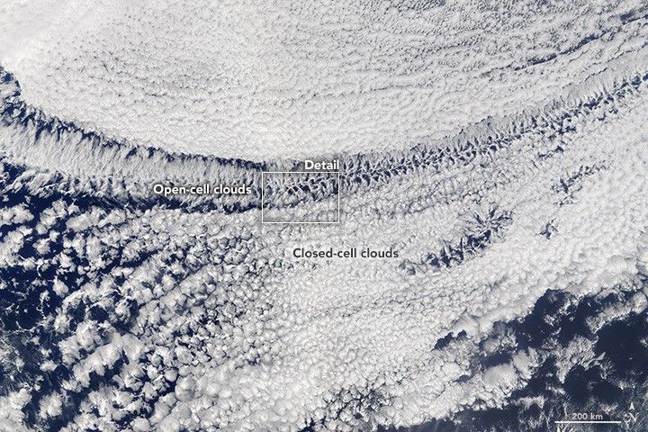
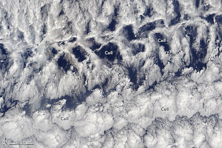
The cleanest case is mesoscale cellular convection — the honeycomb of open and closed cells that stratocumulus decks form over cool oceans, photographed from orbit on almost any marine satellite pass. Closed cells are cloudy centres ringed by clear subsiding edges; open cells invert the pattern, with clear centres ringed by cloudy walls. The cells are strikingly regular and strikingly wide: typical cell diameters run 10–50 km over a boundary layer only 1–2 km deep, an aspect ratio of 15–30. This is the standing anomaly. Classical Rayleigh-Bénard convection selects cells with a horizontal scale only \sim 2–3 times the layer depth — the most unstable mode has a wavelength of order twice the depth. Atmospheric cellular convection is an order of magnitude wider than that, and the discrepancy — the mesoscale cellular convection aspect-ratio problem — has no fully settled explanation. Cloud-top radiative cooling, drizzle, and large-scale subsidence all push toward larger cells, but none cleanly delivers a factor of ten.

The framework reads the cell size as substrate-organized rather than depth-set. The convective overturning supplies the energy; the substrate’s preferred lattice supplies the lateral spacing, the same way it supplies the suction-vortex spacing in a multi-vortex tornado. The substrate’s native packing is Tkachenko’s triangular vortex lattice; the convection cells are its dual, which is exactly why closed-cell decks are famously hexagonal. If the lateral scale is substrate-set, it should decouple from the boundary-layer depth rather than tracking it as Rayleigh-Bénard requires — which is the precise shape of the observed anomaly.

The lateral scale of mesoscale cellular convection should decouple from the boundary-layer depth, and the cells should prefer hexagonal packing. Standard convection ties horizontal cell scale to layer depth (aspect ratio \sim 2–3); the observed 15–30 is the standing anomaly. The framework reads the lateral scale as substrate-lattice-organized rather than depth-controlled, so it predicts (i) cell diameter should correlate only weakly with measured boundary-layer depth across a large stratocumulus sample — the aspect ratio should vary widely rather than sitting near a depth-fixed constant — and (ii) the hexagonal-packing preference should be statistically stronger than pattern-formation models predict for the observed Rayleigh and Marangoni numbers.

When wind shear is added to boundary-layer convection, the cells stretch into cloud streets — long parallel rows of cumulus aligned with the mean wind, often running unbroken for hundreds of kilometres. Each pair of adjacent streets is a counter-rotating roll vortex: rising cloudy motion along one line, sinking clear motion along the next, with horizontal roll axes parallel to the shear. This is the feedback-topology pattern laid down in the boundary layer — a co-rotating updraft channel, a counter-rotating boundary, the pair repeating across the sky. The street spacing is set by the roll diameter, typically 2–8 km for a 1–2 km boundary layer, and the framework reads it the same way it reads the cellular-convection cell size: substrate-organized, with a floor at R_\text{cross}^\text{air} for boundary-layer eddy parameters (\nu_\text{eddy} \sim 10–50 m²/s, \omega \sim 10^{-3} rad/s gives R_\text{cross}^\text{air} \approx 0.4 km, comfortably below the observed spacing) and a preference for the regular periodic packing the lattice favours.

Anton Yankovyi, CC BY-SA 4.0 https://creativecommons.org/licenses/by-sa/4.0, via Wikimedia Commons

Mammatus — the pendulous lobes that hang from the underside of a thunderstorm anvil — are the riskiest and most intriguing case. Unlike cellular convection and cloud streets, mammatus has no settled mechanism at all: the meteorological literature carries close to a dozen competing hypotheses (cloud-base detrainment instability, evaporative cooling, gravity waves, Rayleigh-Taylor and Kelvin-Helmholtz variants), with no consensus. What every mammatus field shares is a strikingly regular lobe size and spacing — smooth pouches \sim 1–3 km across, packed at comparable separation across the whole anvil base. The framework’s reading is the obvious one given everything above: the lobe spacing is a substrate-organized lattice scale, the lobes packing at a preferred separation the same way suction vortices and convection cells do. This reading is qualitative — the lobe rotation rate and the relevant eddy viscosity are poorly constrained — but mammatus offers an unusually clean test precisely because mainstream theory makes no firm spacing prediction, so any substrate-fixed regularity would be a clear signal rather than a contested one.

Cloud-street spacing and mammatus lobe spacing should show a lower edge near R_\text{cross}^\text{air} and regular (periodic for streets, polygonal for lobes) packing, rather than the smooth, depth-controlled distribution standard convection predicts. For cloud streets the test is roll spacing against boundary-layer depth across many soundings, looking for a floor and a packing regularity that survives variation in depth. For mammatus — where mainstream theory makes no firm spacing prediction at all — the test is whether lobe size and spacing cluster tightly across events with very different parent-storm parameters; a substrate-fixed regularity would be a clean signal precisely because no competing theory predicts one.

NoteWhat the framework does not claim for clouds

It does not claim the sharp edge of an ordinary cloud — that is a saturation phase boundary, fully explained by Clausius-Clapeyron and the lifting condensation level. It does not claim why clouds form, where they form, or how much they rain. It does not predict the cell size, street spacing, or lobe spacing from first principles — the substrate elasticity for moist boundary-layer air is no more derivable here than it is for the planetary circulation. The claim is narrow and structural: wherever moist convection organizes into a repeating pattern, the pattern’s spacing should be substrate-set rather than depth-set, with a floor at R_\text{cross}^\text{air} and a preference for triangular/hexagonal packing — the same lattice fingerprint asserted for suction vortices, now in fair-weather and anvil clouds.

Ball Lightning as Atmospheric Modon

Ball lightning is the atmosphere’s most stubborn substrate-shaped mystery. The phenomenon has been reported for centuries: a luminous sphere, typically grapefruit-to-basketball-sized (\sim 10–50 cm diameter), persisting for seconds to occasionally minutes, often appearing during thunderstorms but sometimes not, sometimes passing through closed windows or walls without damage, sometimes terminating in an explosion, sometimes simply fading. Reproduced reports from credible witnesses number in the tens of thousands. Reproducible laboratory analogs exist but only briefly — Kapitsa-style microwave-cavity discharges, Bostick-style plasmoid ejections, and recent silicon-vapor “burning ball” experiments — none lasting more than fractions of a second.

The theoretical landscape is a patchwork. Models include thermochemical (burning silicon vapor from lightning-struck soil), electromagnetic (trapped microwave cavity resonances), plasmoidal (self-confined toroidal plasma vortices, Hill-Bostick-Wells), maser-bubble (Handel-Leitner population inversion), antimatter (Ashby-Whitehead), and several others. None has gained broad acceptance because none predicts the full phenomenology — long lifetime, ability to penetrate dielectrics, internal energy density, and apparent insensitivity to surrounding air composition.

The substrate framework reads ball lightning as the atmospheric analog of a Gulf Stream ring: a self-bound counter-rotating coherent vortex in a fluid (here, ionized air), stabilized by substrate elasticity against the dissipation it would otherwise experience. The toroidal-plasmoid models (Hill 1894; Bostick 1957; Wells & Schmieder) had the right topology — a counter-rotating ring of current-carrying plasma — but lacked an explanation for why such a structure would persist in atmospheric air, where standard MHD predicts decay timescales of milliseconds. The substrate provides the missing piece: once a counter-rotating ring forms above R_\text{cross}^\text{air} (at the relevant rotation rate and turbulent eddy viscosity), the structure substrate-locks and persists for a time set by the substrate-locking number N_\text{lock} rather than by ohmic or viscous dissipation alone.

For a 20 cm ball-lightning radius, plasma rotation \omega \sim 10 rad/s, and turbulent eddy viscosity \nu_\text{eddy} \sim 1 m²/s (appropriate for a hot ionized plasma in air),

R_\text{cross}^\text{air} = \sqrt{\frac{1}{0.3 \times 10}} \approx 0.58\;\text{m}

The 20 cm structure sits below the floor — which is exactly the right qualitative result: ball lightning is marginal, often forms then dissipates within seconds, and is observed primarily at the upper end of the size range (toward 50 cm to 1 m) where it sits closer to the locking floor. Reports of “large” ball lightning (\sim 1 m) are rarer but disproportionately associated with long lifetimes — consistent with the substrate-locking interpretation. The smallest reported ball lightning (\sim 5 cm) is shorter-lived; the substrate cannot lock it efficiently.

Figure 6: Ball lightning as a substrate-locked atmospheric modon. (A) Anatomy: the visible glow is a thin co-rotating plasma dress of ionized air wrapped around a substrate core where the rotational energy actually lives, with a counter-rotating ring (the Hill–Bostick–Wells plasmoid topology) drawn as a counter-rotating \pm\omega dipole. Standard MHD predicts ohmic and viscous decay in milliseconds; once the structure substrate-locks above R_\text{cross}^\text{air} it persists for seconds to minutes, with a lifetime set by the substrate-locking number N_\text{lock} — the same self-bound coherent vortex as a Gulf Stream ring, here in glowing ionized air. (B) The size window: on a log diameter axis the substrate-locking floor R_\text{cross}^\text{air}\approx 0.58 m sets where structures can lock; reports cluster in a sweet spot of \sim 10–50 cm just below the floor (marginal, short-lived), there is a lower-edge cutoff near 5–15 cm below which the substrate cannot lock, the rare large balls (\sim 0.5–1 m) sit at the floor and are disproportionately long-lived, and above \sim 1–2 m a self-shedding ceiling sets in. (C) The contested dielectric-penetration reading: if ball lightning really passes through a closed window, the framework reads the rotational energy as stored in the substrate — present on both sides of the wall — so the substrate-coupled rotation passes straight through while the thin air-plasma dress, which cannot, is shed at the glass and re-formed on the far side, because the wall’s chemical bonding lattice does not couple to the substrate rotation.

NoteThe status of this reading

The substrate interpretation of ball lightning is heuristic, not derivational. It assumes ball lightning is approximately a Hill-Bostick toroidal plasmoid (the framework’s natural reading, but contested in the BL literature), and applies the water-chapter’s R_\text{cross} formula to atmospheric plasma parameters that are themselves poorly constrained from BL observations. The qualitative result — that BL sits near the substrate-locking floor, with larger and slower-rotating balls preferentially long-lived — is consistent with the empirical distribution but not yet a sharp prediction. What the framework offers is the first physical reason for BL’s narrow size distribution: there is a floor below which BL cannot substrate-lock, and a self-shedding limit above which the structure carries too much energy to remain coherent. The middle band (\sim 10–50 cm) is the observed sweet spot.

The substrate reading does not by itself explain BL’s reported ability to pass through dielectric walls without damage. That phenomenology — if real and not a perceptual artifact — would require the BL’s energy to be dominantly stored in the substrate rather than in the air plasma, with the air-plasma component being a visible co-rotating dress on a primarily substrate-coupled rotation. The framework permits this in principle (a substrate-coherent counter-rotating dipole could couple weakly to air molecules at the dress’s outer boundary, slipping through dielectric structures whose chemical bonding lattice does not couple to the substrate rotation), but the prediction is qualitative and the reported phenomenology is unevenly documented. If BL is reproducibly observed to pass through closed dielectric windows, the substrate framework offers a natural reading; if not, ball lightning is purely a plasma phenomenon with a substrate-aided stability floor.

Ball lightning size distribution should show a substrate-floor cutoff near R_\text{cross}^\text{air} for plasma parameters consistent with thunderstorm chemistry. Statistical analysis of catalogued BL reports (Stephan, Cen Jianyong, and the Russian Geophysics archive) should reveal a lower edge in the size distribution near \sim 5–15 cm, with the long-lived events systematically larger. This is testable against existing catalogues without new observation.

The Polar Vortex and Its Sudden Reversals

Above the winter pole, the lower stratosphere develops a coherent rotation — the polar vortex — a counter-rotating boundary that seals off polar air from mid-latitudes. The vortex spins westward at \sim 40 m/s at \sim 25 km altitude, persists from late autumn to early spring, and is largely responsible for the formation of the springtime ozone hole over Antarctica (polar stratospheric clouds form inside the vortex’s cold isolated air, catalyzing ozone-depleting chemistry). The vortex is the atmospheric analog of the tachocline — a sharp counter-rotating boundary in a stratified rotating fluid.

Sudden stratospheric warmings (SSWs) are the polar vortex’s most dramatic substrate-shaped events. Several times per decade, planetary Rossby waves propagating upward from the troposphere break against the polar vortex, deposit easterly momentum that reverses the vortex’s circulation, and warm the polar stratosphere by 30–50 K in less than a week. The vortex temporarily collapses, splits into two or three sub-vortices, or reverses direction entirely. The 2002 Antarctic SSW (the first observed Southern Hemisphere major warming) and the 2009 Arctic SSW are textbook events. Below the warming, the troposphere subsequently exhibits a tropospheric circulation shift on \sim 1 month timescales (negative phase of the Northern Annular Mode, cold-air outbreaks in mid-latitudes).

The framework reads SSW events as the polar vortex undergoing a substrate-mediated reorganization — a transition between two coherent substrate-locked states. Before the SSW, the vortex is a single coherent rotation with a sharp counter-rotating boundary. After, it is either reorganized into multiple sub-vortices (analogous to vortex shedding in fluid mechanics, but at substrate-organized scales) or it has reversed direction. The transition is sudden rather than gradual because the substrate’s elastic response is bistable: either the vortex is substrate-locked in one configuration or it has flipped to another, with no intermediate configurations that are also substrate-locked. The reversal is, in this reading, the same phenomenon as a magnetic dipole reversal in a planetary dynamo (sudden, irregular, with multipolar transition states), and the planetary Rossby-wave forcing plays the role of the convective perturbation that destabilizes the existing locked state.

Figure 7: The polar vortex and its sudden reversals as a substrate-mediated transition. (A) Anatomy: a polar view of the winter stratosphere in which a coherent westward rotation (\sim 40 m/s at \sim 25 km) is sealed off by a sharp counter-rotating boundary. The framework reads that boundary as substrate-locked — the same sharp counter-rotating boundary in a stratified rotating fluid as the solar [tachocline](solar-stellar-dynamics.qmd) — with the cold isolated polar air inside it seeding the springtime ozone hole, and the whole structure expressing the [feedback-topology](feedback-topology.qmd) architecture (co-rotating disk + counter-rotating boundary). (B) Why the flip is sudden: the substrate’s elastic response is bistable, drawn as a double-well potential with one minimum for the coherent vortex and another for the reversed/split vortex, separated by a barrier with no substrate-locked configuration in between; upward-propagating planetary Rossby waves are the perturbation that pushes the system over the barrier, so the transition must be sudden rather than gradual — there is no smooth, half-reversed equilibrium. (C) The reversal itself: a single coherent vortex splits into two or three sub-vortices in a multipolar transition state and then reverses, exactly as a planetary dynamo reverses its dipole; the envelope plot contrasts the framework’s predicted \sim 1-day step in the vortex mean-flow index against the multi-week smooth exponential decay that gradual Rossby-wave dissipation alone would predict.

The temporal envelope of polar vortex reversal during SSW events should be sharper than gradual Rossby-wave dissipation would predict — closer to a step function in vortex-mean-flow indices than to a smooth exponential decay. The 2009 and 2018 SSWs have hourly-resolution stratospheric reanalysis data; the predicted sharpness signature would be visible as a \sim 1-day characteristic reversal time imposed on top of the multi-week Rossby-wave forcing pattern, rather than the multi-week reversal timescale that purely tropospheric dynamics would predict.

Hunga Tonga and the Atmospheric Drum

On 15 January 2022, the Hunga Tonga–Hunga Ha’apai volcano in the South Pacific erupted with one of the most powerful eruptions of the modern instrumental era. The eruption ejected an umbrella cloud to \sim 58 km altitude (the highest ever observed by satellite), injected an unprecedented amount of water vapor into the stratosphere, and — most remarkably — generated atmospheric Lamb waves that propagated around the Earth multiple times. The leading wave passed each surface barometer on its global circuit at \sim 318 m/s (the speed of sound in the lower stratosphere), with a clean pulse signature visible on instruments worldwide for several days. The 1883 Krakatoa eruption produced an analogous wave that circled the Earth seven times before damping below detection threshold. The Hunga Tonga wave persisted for at least three to four passages with high amplitude.

A Lamb wave is a horizontally propagating acoustic-gravity wave that is non-dispersive at the relevant scales — different vertical modes of the same horizontal frequency travel at essentially the same speed. This makes the wave coherent over global distances: the pulse stays sharp as it circles the Earth, where dispersive waves would smear out within a single transit. The framework reads the Lamb-wave phenomenon as the atmosphere ringing in its lowest-order normal mode — the global atmosphere as a thin spherical shell, with a fundamental period set by the shell’s geometry and the local sound speed.

The substrate’s contribution is structural rather than corrective. The Lamb mode’s sharpness over multiple global transits is more persistent than standard acoustic damping predicts: surface-friction estimates for atmospheric Lamb waves give attenuation e-folding distances of \sim 5–10 Earth circumferences, but the observed Krakatoa and Hunga Tonga events suggest the pulses persist closer to the lower end of this range with internal coherence higher than diffusion would maintain. The framework reads this as the substrate forcing the atmospheric shell’s normal mode to retain coherence, in the same way it forces the Gulf Stream cold wall to remain sharp.

Figure 8: Hunga Tonga and the atmospheric drum. (A) The strike: on 15 January 2022 the volcano erupted in the South Pacific, lofting an umbrella cloud to \sim 58 km (the highest ever observed by satellite) and launching a Lamb-wave pulse that spread across the globe, reconverged at the antipode, and circled the Earth multiple times — the leading front passing each surface barometer at \sim 318 m/s with a clean, sharp signature on every passage (Krakatoa 1883 circled seven times; Hunga Tonga at least three to four with high amplitude). (B) The reading: the atmosphere struck like a drum rings in its normal modes, which is the same physics as the global atmosphere treated as a thin spherical shell sounding its lowest-order mode, with a fundamental period set by the shell’s geometry and the local sound speed. Because the Lamb wave is non-dispersive — all vertical modes of one horizontal frequency travel at the same speed — the pulse stays a sharp spike around the whole planet, where a dispersive packet would smear out within a single transit. (C) The substrate’s contribution: a plot of pulse coherence against Earth circumferences traveled in which standard linear acoustic theory predicts the pulse smearing and e-folding away within \sim 5–10 circuits, while the observed Krakatoa and Hunga Tonga pulses sit above that decay on a substrate-held coherence floor — the same structural sharpening that holds the Gulf Stream cold wall sharp, here forcing the global atmospheric mode to retain coherence past what diffusion would maintain.

The dispersion and attenuation of major-eruption atmospheric Lamb waves should show a substrate-mediated coherence floor that is invisible to standard linear acoustic theory. The 2022 Hunga Tonga event produced the highest-quality global Lamb-wave dataset ever recorded; a careful re-analysis comparing observed attenuation and dispersion to standard atmospheric acoustic models should reveal a residual coherence consistent with substrate-elastic stiffening at the global mode scale.

The deeper point: a major volcanic eruption is the atmosphere being struck like a drum. The drum rings in its normal modes. The substrate, present everywhere the atmosphere is, contributes a structural sharpening to the lowest-order mode the same way it sharpens the planetary three-cell circulation. Each is the atmosphere assuming the substrate’s preferred geometry under coherent forcing.

Transient Luminous Events and the Substrate Peeking Through

Above thunderstorms, a family of brief luminous phenomena — red sprites, blue jets, elves, halos, gigantic jets — connects tropospheric lightning to the upper atmosphere and the ionosphere. Sprites are red columns and tendrils at 50–90 km altitude, lasting \sim 3 ms after a positive cloud-to-ground lightning stroke. Blue jets shoot upward from cloud tops to \sim 50 km altitude in cone-shaped streamers, lasting tens to hundreds of milliseconds. Elves are expanding luminous rings at the ionosphere (\sim 90–100 km), driven by lightning EMP. Halos are diffuse glows at \sim 80–85 km surrounding the centers of strong lightning strokes.

These are catalogued and partially explained by atmospheric electrodynamics: the electric field of a cloud-to-ground discharge propagates upward through the increasingly tenuous atmosphere, exceeds the local breakdown threshold at high altitude where the air density is low, and excites molecular nitrogen and oxygen into characteristic emission lines (red from N_2 first positive system in sprites, blue from N_2^+ in jets). The lightning chapter treats the underlying substrate physics of the 300 keV modon-shedding threshold and the substrate channel structure that lightning follows.

What this chapter adds is a brief observation: TLEs are the visible bridge between the substrate’s lower-atmosphere window (lightning) and the substrate’s space window (solar system boundaries). The phenomena occur at altitudes where the air density is low enough that the substrate’s coupling to bulk gas is weak, but where modon emission from runaway electrons is still possible. Sprites and jets are, in this reading, the same kind of substrate-mediated emission as the lightning bolt itself, but propagating into a regime where the air is too thin to support a continuous discharge channel, so the substrate response shows up as diffuse glows and brief filamentary structures.

The framework’s prediction here is the same as in the lightning chapter: sprite emission should include a substrate-driven enhancement at energies above the 300 keV threshold, and the spatial pattern of sprite filaments should align with the substrate’s domain structure rather than with the local electric field alone. The TLE community has begun searching for hard-X-ray and gamma-ray correlations with TLEs (the ASIM mission on the ISS, the TARANIS-style instruments) and the data are still preliminary; if substrate-shed gamma rays appear in TLEs at the predicted threshold, the substrate’s signature will have been confirmed in an entirely separate atmospheric regime from cloud-to-ground lightning.

Figure 9: Transient luminous events as the substrate peeking through. (A) The TLE family drawn as an altitude cross-section from the thundercloud to the ionosphere: a positive cloud-to-ground stroke launches blue jets in cone-shaped streamers up to \sim 50 km, red sprites as columns and tendrils between \sim 50 and 90 km (\sim 3 ms after the stroke), a diffuse halo glow at \sim 80–85 km, and expanding elves rings at the ionosphere (\sim 90–100 km), with gigantic jets bridging cloud top to ionosphere in one event. The settled electrodynamics — the +CG field exceeding breakdown in ever-thinner air and exciting N_2 (red) and N_2^+ (blue) — is preserved; what the framework adds is that TLEs are the visible bridge between the substrate’s [lower-atmosphere window](lightning.qmd) and its [space window](solar-system-boundaries.qmd). (B) The reading: against a vertical air-density column that thins from dense ground air to near-vacuum ionosphere, the dense low air sustains a continuous discharge channel — the lightning bolt — while in the thin air above, too tenuous to hold a channel, the same substrate-mediated modon-shedding emission can only leak out as diffuse glow and brief filaments. (C) The energetic tell: the standard breakdown spectrum cuts off above tens of keV, but the framework predicts a substrate-shed hard-X-ray / \gamma-ray excess above the 300 keV modon-shedding threshold (the regime ASIM and TARANIS-class instruments are now searching), and sprite filaments should track the substrate’s domain lattice rather than fanning with the local electric field alone.

What Air Predicts

Prediction	Substrate origin	Test
Tropopause and stratopause sharpness floor at substrate width range	Counter-rotating substrate boundaries between atmospheric circulation cells	Radiosonde and limb-sounding statistics on inversion thickness across conditions
Number of meridional cells scales with substrate-stiffness/thermal-forcing ratio across planets	Substrate inserts counter-rotating intermediate cells	Comparative survey of Earth, Mars, Jupiter, Saturn atmospheric circulations
MJO amplitude distribution bistable around the Rostami-Zeitlin threshold	Substrate-locking threshold: convergence-and-lock vs Gill-scenario radiation	Wheeler-Hendon RMM and OMI index PDF for a gap near \Delta H/H \approx 0.15 rather than a smooth tail
MJO genesis follows R-Z onset criteria — circular tropospheric depressions of \sim L_d scale, 0.15–0.20 amplitude	Equatorial modon as substrate-locked L-R dipole; large-aspect-ratio anomalies decompose into Rossby packets	ERA5 reanalysis composite of pre-onset MJO events; correlation of subsequent modon formation with initial-depression geometry
MJO active-phase tropical cyclone genesis preferentially clusters at modon leading edge	Atmospheric analog of suction-vortex shedding, scaled to planetary modon	Historical cyclone tracks vs contemporaneous MJO RMM phase and modon-envelope position
Hurricane eyewall-replacement radii cluster at discrete substrate-organized scales	Substrate-preferred lattice for nested coherent rotations	Statistical analysis of historical eyewall-replacement events vs. continuous-prediction baseline
Hurricane minimum size \sim 1 km from R_\text{cross}^\text{air} for cyclonic parameters	Substrate-locking floor in atmospheric vortices	Catalogue of smallest tropical cyclones; floor should align with prediction
Multi-vortex tornado suction-vortex spacing \sim 10–30 m with triangular-lattice preference	Substrate’s Tkachenko lattice asserted at atmospheric scale	Doppler-radar reconstructions (El Reno 2013, Bridge Creek 1999); spacing and geometry statistics
Mesoscale cellular convection scale decouples from boundary-layer depth; hexagonal packing	Substrate lattice sets lateral cell spacing, not convective depth	Satellite stratocumulus survey: cell-diameter vs boundary-layer-depth correlation and hex-packing statistics
Cloud-street and mammatus spacing show R_\text{cross}^\text{air} floor and regular packing	Substrate-locking floor + Tkachenko lattice in moist convection	Roll-spacing vs sounding depth; mammatus lobe-spacing clustering across storms
Ball lightning size distribution shows substrate-floor cutoff near R_\text{cross}^\text{air} for thunderstorm plasma	Substrate-locked atmospheric modon analog	Statistical analysis of catalogued BL reports for lower edge and lifetime-size correlation
Polar vortex SSW reversals proceed as sharp \sim 1-day transitions, not gradual decay	Bistable substrate-locked states; reversal between locked configurations	Hourly-resolution reanalysis of 2009/2018 SSW events for envelope sharpness
Atmospheric Lamb-wave attenuation slower than linear-acoustic prediction	Substrate-stiffening of lowest-order global atmospheric mode	Re-analysis of Hunga Tonga 2022 barometric data for residual coherence
Sprite and TLE emissions include substrate-driven gamma-ray component above 300 keV threshold	Same modon-shedding mechanism as lightning, in low-density regime	ASIM and TARANIS-class hard-X-ray observations of TLE-correlated events

Connections

This chapter sits at the intersection of several established framework threads:

• The feedback topology chapter supplies the architecture (co-rotating disk + counter-rotating boundary + polar exits + radiated residual) that the planetary three-cell circulation, the hurricane, and the polar vortex all express at their respective scales.
• The water chapter supplies the R_\text{cross} formula and the substrate-locking number N_\text{lock}, which this chapter applies to atmospheric eddy viscosities and rotation rates. It also supplies the three-step convergence-and-lock mechanism for modon formation, which the equatorial modon / MJO section above applies to moist tropical air with the planetary vorticity gradient and condensation-driven mass convergence playing the roles of the substrate’s chirality-coherent sheets and atomic boundary collapse. The mechanism is the same; only the host medium and the convergence driver have changed.
• The fire chapter establishes the firestorm as the local atmospheric assertion of the substrate’s preferred geometry. Hurricanes and tornadoes are the same architecture expressed in the absence of fire — pure rotational organization in moist air.
• The lightning chapter treats the substrate becoming visible in atmospheric plasma above the 300 keV threshold. This chapter is its lower-energy complement: the substrate becoming structurally relevant whenever air organizes itself into coherent rotation, even far below the modon-shedding regime.
• The gaia substrate chapter provides the nested-feedback architecture in which Earth’s atmospheric layering sits. The stacked atmosphere is one of the seven layers of the Gaia stack; air-in-the-substrate adds the structural reading of why the layering is sharp.
• The solar-stellar dynamics chapter develops the tachocline as the stellar analog of the polar vortex — a thin counter-rotating boundary in a stratified rotating fluid, sharpened by substrate elasticity in both cases.
• The solar system boundaries chapter treats Jupiter’s banded atmosphere and the Great Red Spot as long-lived substrate-organized vortex systems in gas-giant atmospheres — Earth’s tornadoes and hurricanes are the terrestrial analogs at smaller scale and shorter lifetime.
• The bridge equation fixes \alpha_{mf}, \xi, c_T, 0.776\,c — every prediction in this chapter draws on these and adds no new parameters.

What the Four Elements Together Reveal

Water is the substrate’s preferred fluid, the medium it organizes most easily at every scale from the molecule to the ocean basin. Ice is the substrate template made visible in a crystalline solid, the hexagonal sheet structure locked into molecular geometry. Fire is the substrate’s surface activity made visible whenever boundaries reorganize at temperatures the lattice can ignore. Air is the substrate’s quietest collaborator — a medium so thin that the substrate has almost no mechanical grip on it, present everywhere weather happens, structurally relevant only where the atmosphere organizes itself into coherent rotation but absolutely necessary there.

The four elements arrange themselves along a single axis of substrate participation. Ice is fully locked — the substrate template visible in every snowflake and glacier. Water is soft-locked — the substrate organizing mesoscale flows without rigidifying them. Fire is surface-active — the substrate at the boundary of materials, where chemistry reorganizes and the lattice averages over. Air is structurally permissive — the substrate’s grip too weak to constrain bulk dynamics, but always present to sharpen boundaries and stabilize coherent vortices when the atmosphere produces them. Read through the substrate ladder’s two poles, all four elements sit on the lock side: each is matter binding to the substrate’s preferred order, differing only in how completely. None reaches for the anti-lock pole — the deliberate refusal of resonance seen in phyllotaxis, the retinal cone mosaic, the resting cortex, and the genetic code — because that pole is the signature of a structure that must stay distinguishable from its neighbours, and in this paper its witnesses are all living systems. The four elements are the lock pole in four strengths.

Earth — the remaining classical element — would complete the picture as the regime where chemistry and mechanics dominate and substrate participation is most thoroughly buried. Rocks, soils, and minerals are the substrate’s least transparent host: the lattice template is there (Ice Ih’s hexagonal symmetry inherited from the substrate sheet structure shows up in many silicate minerals, and the aromatic rings chapter’s 36 kcal/mol topological energy is a feature of much organic geochemistry), but it is mostly invisible because most everything happens at scales where chemistry has long since taken over. The framework’s window onto Earth-the-element will be subtle — soft compared to fire’s vivid color, water’s coherent currents, ice’s crystalline templates, or air’s rotating storms.

Together the elements span the temperature axis from the substrate’s coldest expression (ice, fully locked) through its room-temperature expressions (water, air, earth) to its hottest expression (fire, surface tearing). Each is a different stance the substrate takes toward the matter occupying it, and reading them together is the closest the framework can come, in the everyday world, to seeing the medium that makes everyday physics work.

Footnotes

1. Two papers establish the equatorial modon: Rostami, M. and Zeitlin, V., “Eastward-moving convection-enhanced modons in shallow water in the equatorial tangent plane,” Physics of Fluids 31, 021701 (2019) constructs the analytical asymptotic solution and confirms numerically that it is an attracting solution of the full nonlinear system; “Geostrophic adjustment on the equatorial beta-plane revisited,” Physics of Fluids 31, 081702 (2019) shows the modon forms naturally from moist-convective adjustment of a localized pressure depression above a sharp threshold in initial amplitude.